Microsoft Excel is one of the most complete options to work with data in a much more centralized way of each one of them. Excel has hundreds of functions and formulas designed for a much more complete work and one of them is to use formulas to determine the amortization table of a loan, remember that amortization consists of gradually reducing a debt or a loan with periodic payments, the amortization table in Excel will give us a global detail of each of the payments until we pay in full said credit..
Amortization table requirements
To correctly create the amortization table in Excel it is necessary to have the following:
- Amount of the credit: we must know exactly the amount of the loan, this is the value that the bank finally gives us.
- Interest rate: knowing the interest rate charged by the financial institution is a key aspect, as a general rule the interest rate is deducted annually.
- Number of payments: knowing the number of payments allows us to know how long we will be linked to the financial entity, these payments are represented in monthly periods such as 12, 24, 36, 48, etc.
Data
In our case we handle the following data:
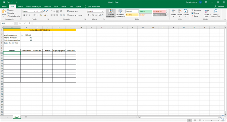
With these data we are going to see how to make an amortization table Excel fixed fee in detail in text and video.
To stay up to date, remember to subscribe to our YouTube channel! SUBSCRIBE
1. Calculate Excel fixed fee
Step 1
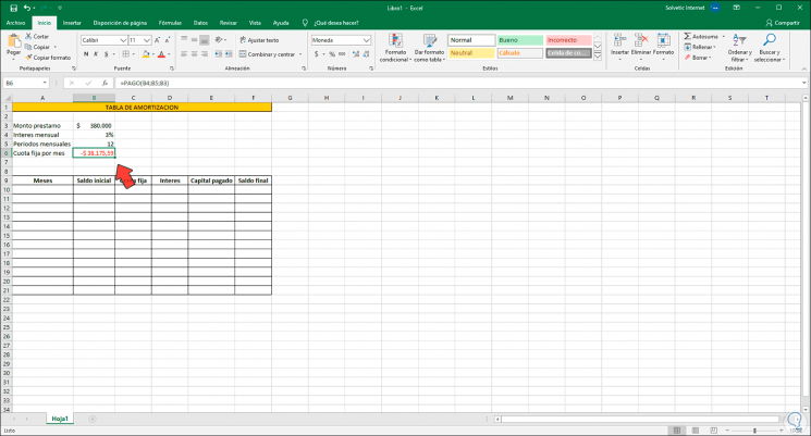
The first step to take will be to calculate the fixed fee that we must pay, for this we go to the cell "Fixed fee per month" and we will use the formula "Payment" as follows:
= PAYMENT (B4; B5; B3)
Step 2
The following values have been defined in it:
(monthly interest; number of months; loan amount)
Step 3
The default result will give a negative number:
Step 4
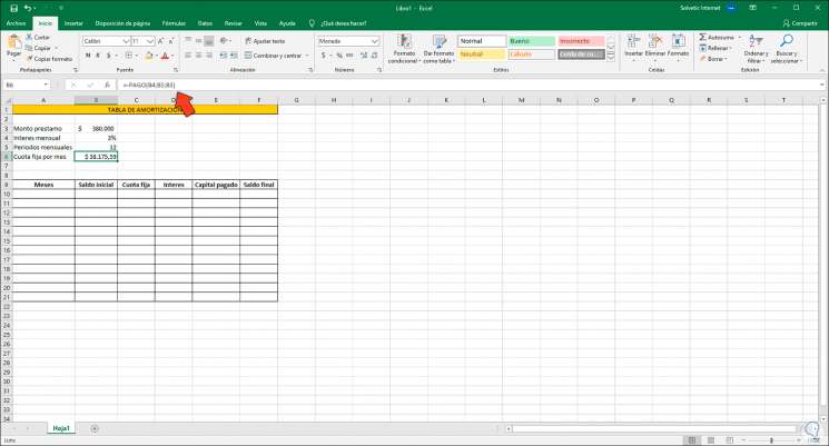
For the amortization table to work correctly, we must convert the negative value to positive, for this we enter a sign - before the "payment" function:
= -PAYMENT (B4; B5; B3)
Step 5
Now the number will be positive:
2. Set up depreciation table Excel
Step 1
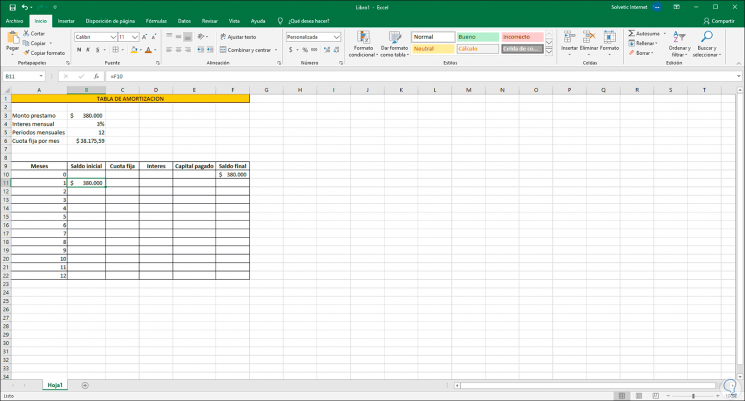
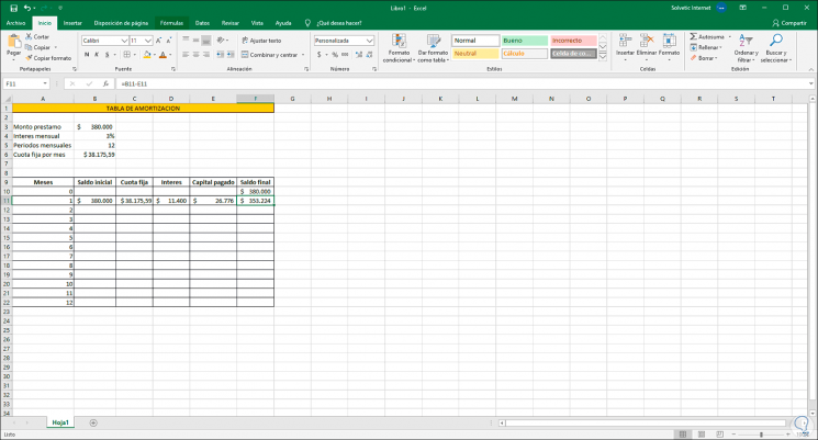
It is time to manage the table to know in detail the values to be paid and collected, the first thing will be to enter the months, as in this case they are 12, we enter from period 0 to 12 (in period zero we enter the disbursement of the credit).
In the Final Balance cell we can reference the cell where the loan amount has been entered:
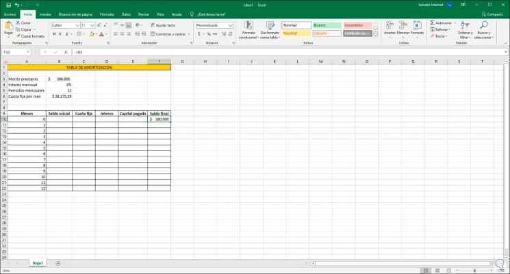
Step 2
Now, we reference cell F10, which is where we have entered the loan amount, into cell B11 associated with the initial balance of the loan:
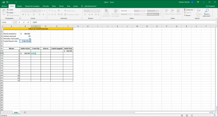
Step 3
In the section "Fixed fee" we have already defined the monthly fixed value, this value will not change throughout this section, in cell C11 we enter the reference of the cell where the fixed fee has been defined (B6), we must convert this cell in absolute reference so that its value does not change as we drag the cell down, when entering the reference we press the F4 key and we will see the $ sign next to the column and the cell:
= $ B $ 6
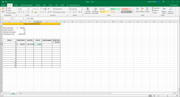
Step 4
Now we calculate the monthly interest, for this we multiply the initial balance by the interest rate charged with the following formula in this example:
= B11 * $ B $ 4
Note
cell B4 has been left absolute because it is a fixed value.
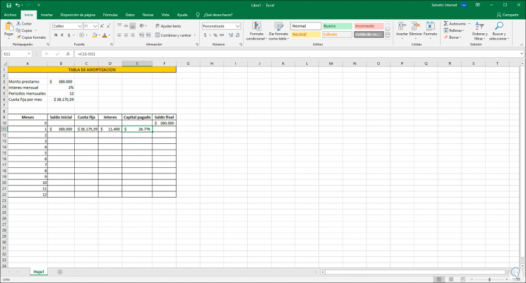
Step 5
Now it is time to calculate the capital paid which is the difference between the fixed installment minus the monthly interest paid, we will use the following formula:
= C11-D11
Step 6
The result of this is what will be reduced from the initial debt:
Step 7
To define the final balance we will take the initial balance minus the paid-in capital:
= B11-E11
Step 8
Finally, we simply select the cells of the amortization table and drag them from the lower right corner to the last defined period so that the values to be paid are displayed:
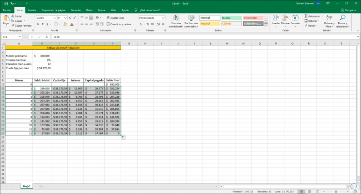
With this simple method we can create an amortization table as an example in Excel and with it, take precise control over the values that we must pay month by month and know with certainty whether or not the agreed conditions are met.