Microsoft Excel 2019 is the new Office commitment to facilitate and centralize the management of data independent of its type, remember that in Excel we can work with numerical, date, text and more data which were managed in a dynamic way thanks to the functions, formulas and tools integrated within the application.
One of the most common ways, and one of the most obscure sounds in Excel 2019, is to manage and visualize the data through the pivot tables..
With the creation of a pivot table it will be possible to summarize, analyze, explore and present in a much more organized way the summary data of the selected range. Alternatively, we can combine dynamic graphs which are a complement to the dynamic tables which allow integrating visualizations to the summary data in a dynamic table and thus have a clearer perspective of the comparisons , patterns and trends of the data.
With dynamic tables it will be possible to connect to external data sources such as SQL Server tables, SQL Server Analysis Services cubes, Azure Marketplace, Office data connection files (.odc), XML files, Access databases and files of text in order to create pivot tables or use existing pivot tables and from there create new tables..
Advantage
Among the great advantages of using a pivot table we have:
- Move rows to columns or columns to row, called pivot action, in order to analyze different summaries of the source data.
- Consult large amounts of data.
- Expand and collapse data levels to highlight the results displayed.
- Access subtotals and sums of numerical data, summarize data by categories and subcategories, or create custom calculations and formulas as necessary.
- Filter, sort and group the most relevant subsets of data.
- Submit reports online or in print.
TechnoWikis will explain through this tutorial how to create a pivot table in Microsoft Excel 2019.
1. How to create a pivot table in Excel 2019
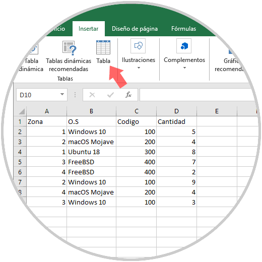
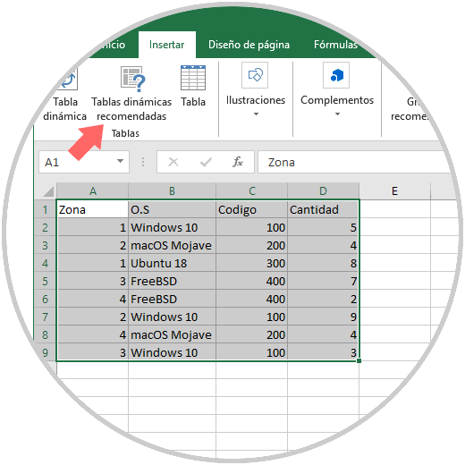
As of the 2013 edition of Excel, Office integrated an option called Recommended Pivot Tables which we found in the Insert menu and in the Tables group:
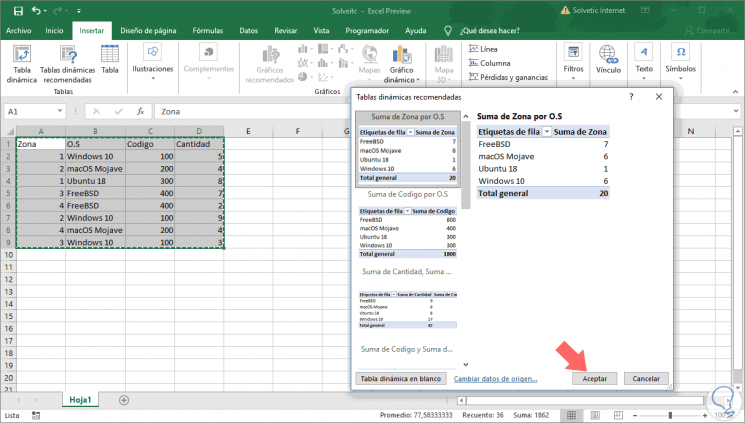
This recommended pivot table is a pre-designed summary of the data that Excel recommends based on the selected information, it is practical for a quick analysis of the information..
Step 1
To make use of this function integrated in Excel 2019, we must select the data to be represented in the pivot table and click on the Dynamic tables button recommended in the Tables group and the dynamic table that Excel 2019 considers adapts to the data taken will automatically be displayed :
Step 2
If we click on the Accept button this pivot table will be inserted in the active sheet:
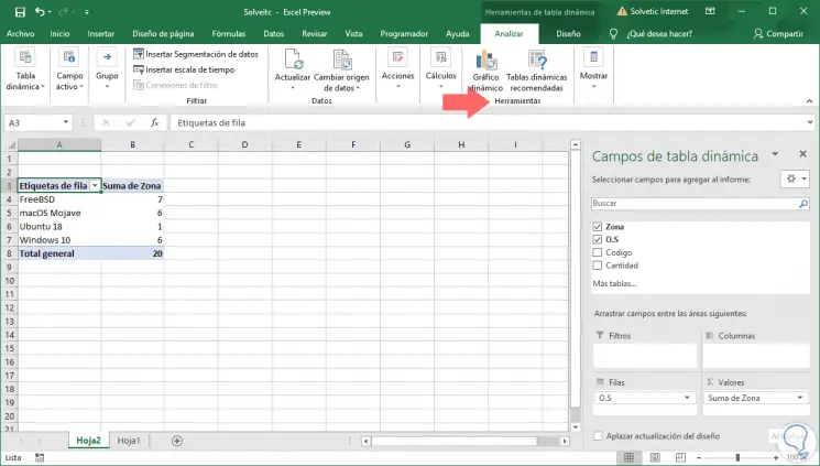
Once integrated, the Pivot Tools menu will be activated from where it will be possible to make all the changes we consider necessary.
Actions in a pivot table
When we work with a pivot table it will be possible to carry out actions such as:
Explore the selected data with the following parameters:
- Expand and collapse the data and display the underlying details that belong to the values.
- Sort, filter and group fields and other elements.
- Modify summary functions and add custom calculations and formulas.
Edit the layout of the columns, rows and subtotals with actions such as:
- Enable or disable field headers in column and row, or show or hide blank lines.
- Display subtotals above or below rows.
- Adjust column widths when updating.
- Move a column field to the row area or a row field to the column area.
- Merge or divide cells for external elements of rows and columns.
Change the design of the form and the layout of those with functions such as:
- Change the format of the pivot table to Compact, Schematic or Tabular.
- Add, organize or delete fields.
- Change the order of the fields or elements.
Change the display format of blank spaces and errors with values ​​such as:
- Modify how errors and empty cells are displayed.
- Edit the way elements and labels are displayed without data.
In the right side panel we can work various actions on the data, we can see in the bottom sections such as Filters, Columns, Rows or Values, each of these options allows us to visualize and filter the data as necessary.
Step 3
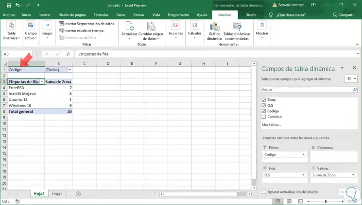
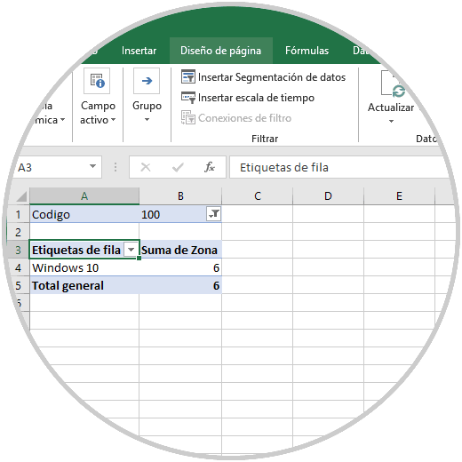
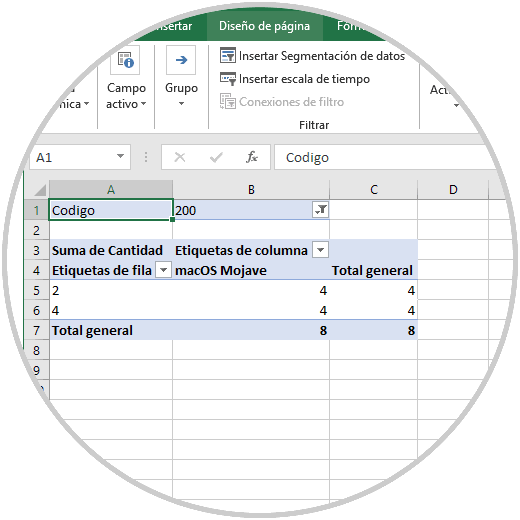
For example, we have added the Code row to the Filter field and we can see that the Filter field is added at the top of the sheet:
Step 4
If we click on that field, the data registered in that section will be displayed and we can click on the option to filter:
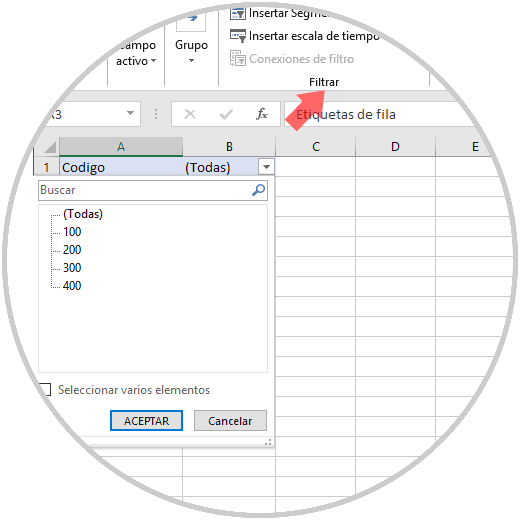
Step 5
Once we select the filter it will be possible to see that the pivot table will only launch the results based on this filter:
Thus, with the recommended pivot tables it will be much simpler to create and manage the data in Excel 2019.
2. How to create a pivot table in Excel 2019 manually
Now, if for some reason we don't like the automatic option integrated in Excel 2019, it is possible to create the pivot table manually from scratch.
Step 1
For this process, we select the range of data to use and from the Insert menu, Tables group, select the PivotTable option:
Step 2
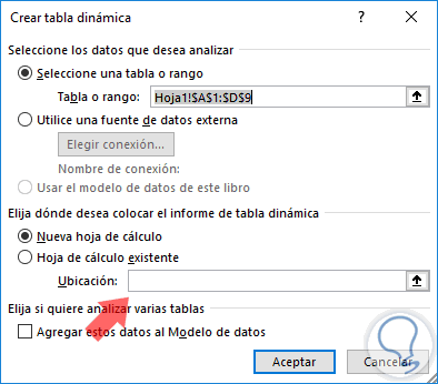
Clicking there will display the following wizard:
Step 3
First, we will see the range of data that we have selected and at the bottom we can define in which location the pivot table will be housed.
The following will be displayed:
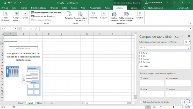
Step 4
On the right side we can drag each row to the field that we consider necessary for the display of the data, for example, if we had rows of values ​​or sum, this should go in the Values ​​section.
Edit
For this case we will edit the following:
- Zone will go to the Rows section
- OS will go to the Columns section
- Code will go to the Filters section
- Amount will go to the Values ​​section
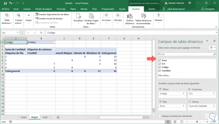
Step 5
With this scheme, it will be possible to filter the desired data and automatically the pivot table will launch the data associated with that filter:
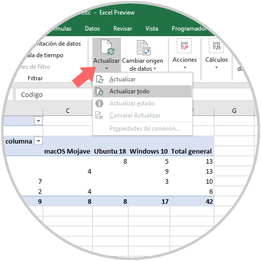
Step 6
If there is any change in the original data, we must go to the Data group and click on Update and there select the correct option:
Step 7
From the Design tab it will be possible to change the way the pivot table looks to cause a greater impact:
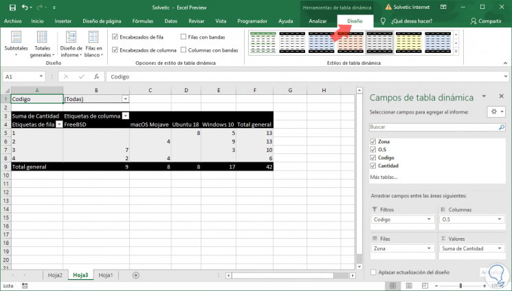
Step 8
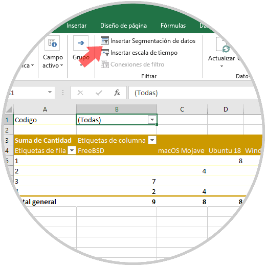
One way to further customize the data in the pivot table in Excel 2019 is by segmenting the data, for this we will go to the Analyze tab and in the Filter group we will see the option Insert Data Segmentation:
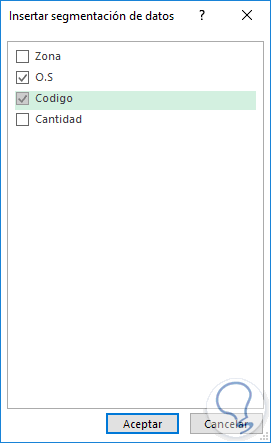
Step 9
The following window will be displayed where we will select one or more parameters to segment:
Step 10
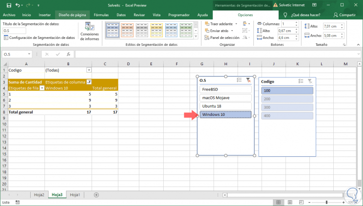
Click on Accept and as a result we will have, in this case, two pop-up windows like this:
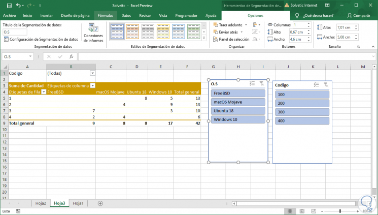
Step 11
There we can click on any of the highlighted values ​​to apply the respective filter:
Step 12
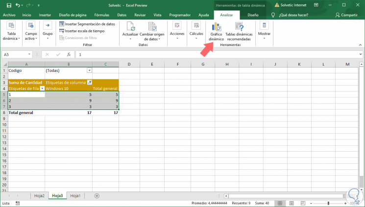
In order to further highlight the registered data, we can insert a dynamic graph with the registered information, for this we select the data to graphs and go to the Analyze tab and in the Tools group we click on the Dynamic Graph option:
Step 13
The following window will be displayed where we select the type of graph to be inserted:
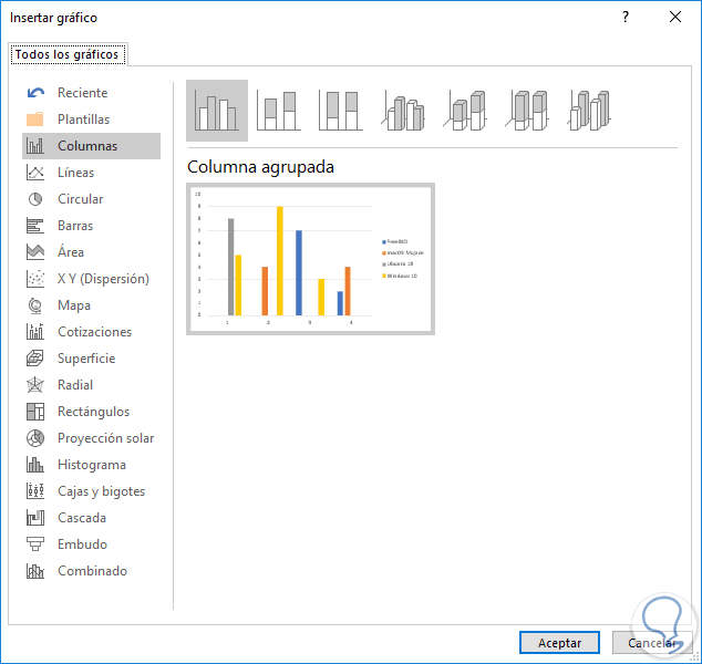
Step 14
Once we click on Accept, the graph will be added and within it we can apply filters based on the selected data:
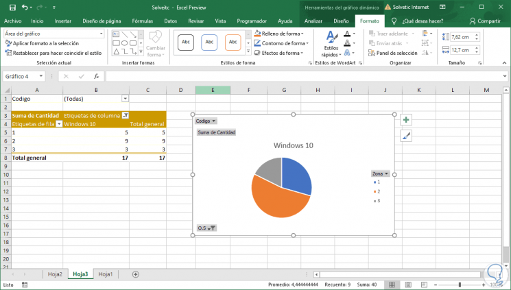
In this way, dynamic tables are one of the best alternatives for working on large amounts of data, simplifying their management and with the multiple tools to present the data in a professional manner.