Financial decisions are an important element of business strategy and planning. But we also have to make a lot of financial decisions in everyday life. For example, if you are applying for a loan, it will certainly be helpful if you know exactly what interest rate you have to pay at your bank. For such cases, Excel offers the INTEREST function, which is specially designed for calculating the interest rate for a certain period of time.
Calculate total interest in Excel
The total return on an investment that has to be paid over a certain period of time can easily be calculated in Excel with the appropriate INTEREST function.
The INTEREST function syntax has the following arguments:
- Interest : This is the interest rate.
- Per : This is the period for which the interest should be calculated.
- Zzr : This argument specifies the length of time over which the respective annuity is paid.
- Bw : This is the capital.
- Zw : This is the future value to be achieved after the last payment and is optional.
- Q : The F indicates when payments are due and can either have the value 0 at the end of a period or 1 at the beginning of a period. This value is also optional.
With these arguments the function looks like this: ZINSZ (Interest; Per; Zzr; Bw; [Zw]; [F]) .
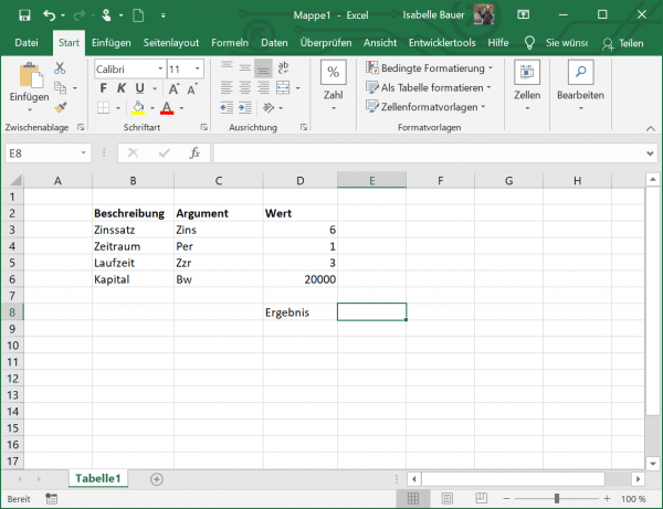
Let us now apply this function to an example. You can see in the figure that the annual interest rate is 6.00%, which is in cell D3. You can enter this as a percentage, as in the example, or as a decimal number. So, if you are making annual payments on a loan with an annual interest rate of 6%, use 6% or 0.06 as the rate. If you make weekly, monthly, or quarterly payments, divide the annual interest rate by the number of payment periods per year. For quarterly payments on a loan with an annual interest rate of 6%, use 6% / 4 for the interest rate.
We have specified 1 as the period, which is in cell D4. The term of the loan is in cell D5 and is 3. So we calculate the interest for 3 years. The initial capital is € 20,000 and is in D6. In summary, we would like to calculate the interest for a capital of € 20,000 in annual payments over 3 years with an interest rate of 6%.
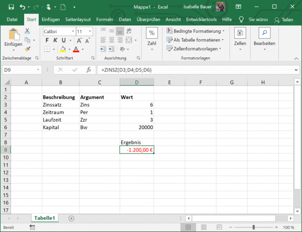
So let's use the formula = INTEREST (D3; D4; D5; D6) . You can see that we did not include the arguments Zw and F in our formula. As a result, both of these are set to 0, which means that the final value of € 0 should be reached and the payments take place at the end of a period.
The result now shows the interest that is due after the first year of payment at an interest rate of 6%..
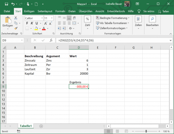
However, if you want to calculate the interest for quarterly payments, for example, you have to adjust the values in your function. For the interest rate argument , divide the annual interest rate by the number of payments per year, assuming that the latter is equal to the number of compounding periods per year. For the Zzr argument, multiply the number of years by the number of payments per year. In our example, the interest rate for quarterly payments is 6% / 4 and the term is 3 * 4.
Let's change the formula accordingly: = ZINSZ (D3 / 4; D4; D5 * 4; D6) .
The result now shows the interest that is due after a quarter.
Calculate the interest rate in Excel
INTEREST is an Excel finance function that determines an interest rate for a specific period on an annuity.
The function syntax is as follows:
- Zzr : This argument specifies the length of time over which the respective annuity is paid.
- Rmz : The fixed payment amount per period that cannot be changed during the term of the annuity. As a rule, it includes capital and interest, but no taxes.
- Bw : This is the current value of the loan or investment.
- Zw : This is the future value to be achieved after the last payment and is optional.
- Q : This indicates when payments are due and can either have the value 0 at the end of a period or 1 at the beginning of a period. This value is optional.
- Estimate : Your guess what the rate might be. If this argument is omitted, the value is set to 10%.
With these arguments, the function looks like this: ZINS (Zzr; Rmz; Bw; Zw; [F]; [estimate]) .
In our example, let's see how to create the INTEREST formula in its simplest form to calculate the interest rate in Excel. So let's say you've taken out a $ 10,000 loan that you want to repay in full over the next three years. You plan to pay 3 annual installments of € 3,800 each. Let us now define the following arguments for the Excel INTEREST function.
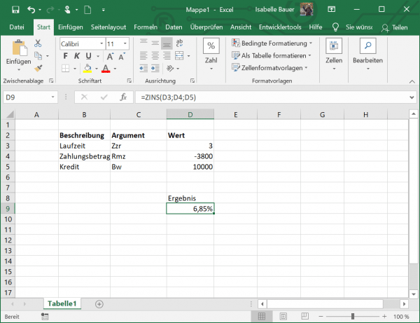
Cell D3 contains the number of payments, i.e. 3. In D4 you can see the payment amount, i.e. -3,800. Make sure that there is a minus in front of the number, otherwise the function will throw an error. You can find the value of the loan in cell D5, which is 10,000. Now use the appropriate formula: = INTEREST (D3; D4; D5) ..
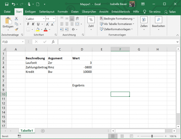
It is assumed that payment should be made at the end of each year, so we can omit the F argument or set it to the default value (0). The other two optional arguments Zw and Estimated are also omitted.
The result now shows that the interest rate is 6.85%.
Calculate compound interest in Excel
The KUMZINZ function calculates the cumulative interest that arises between a certain period of time.
The syntax of the COUNTINST function has the following arguments:
- Interest : This is the interest rate.
- Zzr : This argument specifies the length of time over which the respective annuity is paid.
- Bw : is the capital.
- Period_start : This is the first payment in the calculation.
- Period_End : This is the last payment in the calculation.
- Q : The F indicates when payments are due and can either have the value 0 at the end of a period or 1 at the beginning of a period. In contrast to the first two functions, the value is required here.
With these arguments, the function looks like this: KUMZINSZ (interest; Zzr; Bw; period_start; period_end; F) .
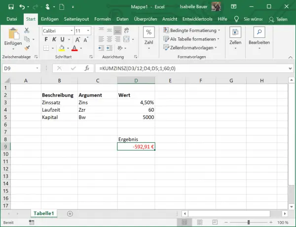
Now imagine a scenario in which you have a capital of € 5,000 in a bank that pays you 4.5% interest per year. You would like to invest in the fixed-term deposit over a period of 5 years. Let us now calculate the compound interest for this period.
In D3 you can see the interest rate of 4.5%. You can see the total number of payment periods in cell D4. Since we calculate for 5 years, this value is 60 (5 years = 60 months). Cell D5 contains the capital amount, i.e. 5,000. Our formula now looks like this: = UPDATE (D3 / 12; D4; D5; 1; 60; 0 ).
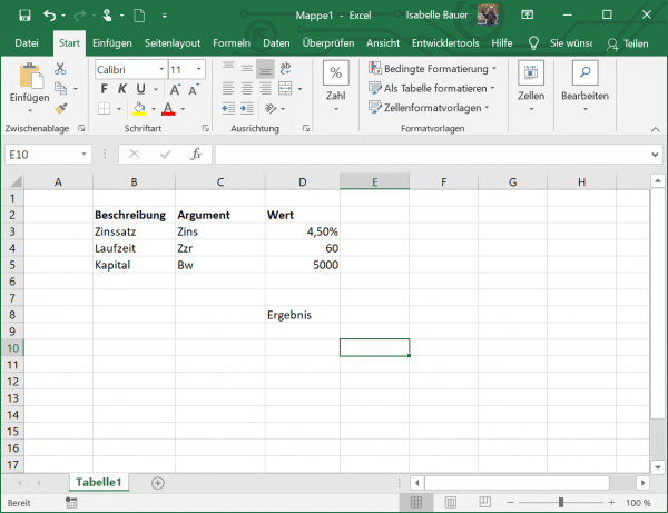
We divide the value in D3 by 12, since 4.5% represents the annual interest, but in this example we calculate in months.
The result now shows the compound interest that you will receive on your capital after 60 months.
