When working with formulas in Excel, one of the most important features in terms of productivity and consistency that we already explained in how to copy and paste formulas in Excel, is the possibility of being able to copy the formulas made in other cells, and to drag formulas when we make data tables..
When we say that it is one of the most important features, it is because in practice, we are going to use copy and paste very frequently to be able to move faster in our work.
When we copy and paste a formula, or drag the formula to other cells, Excel applies table logic, copying the structure of the formula, to fit the destination cell..
For example, when we work in columns, and we carry out a formula in the first row with data referenced to cells that are in the same row, when stretching or copying the formula, this same operation will be carried out, but adapting in each case to reality. of the cell where the formula is to be pasted.
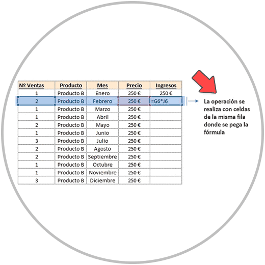
Normally, when we work or are building a data table, some of the operations that we are going to perform, as in the image that we have just shown you, will be between cells that are in the same row..
Thus, as we saw in how to copy and paste formulas in Excel, in a table where we have information that complements the sales that are recorded in a given period of time, one of the actions that we can carry out will be to calculate at the level of row, the income we have had in each period. (In the example each row represents the sales of a month).
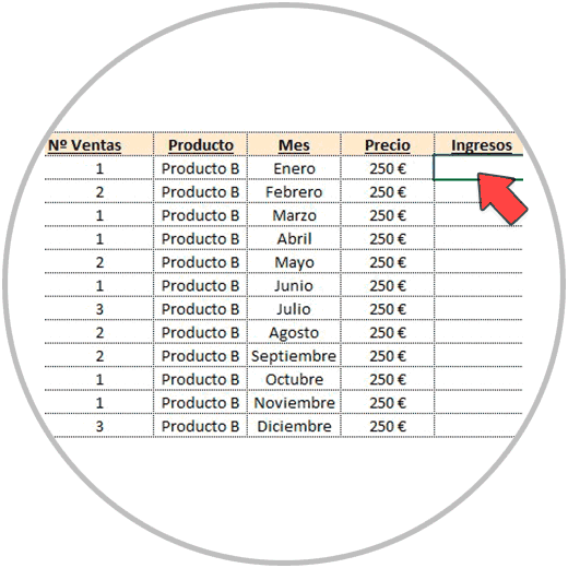
So to calculate the total income, we are going to first calculate by row what the monthly income is, and to carry out this operation we would multiply the number of sales of each row, by its price or unit value.
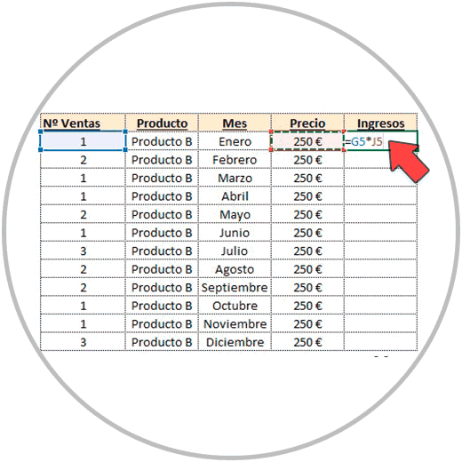
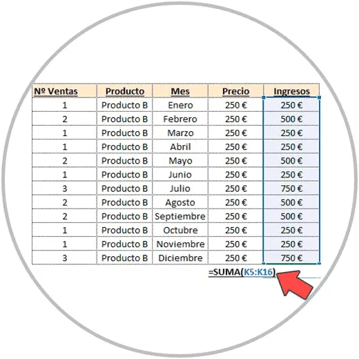
By performing this formula, we can stretch or copy and paste the formula in the rest of the rows of the table, and thus we will have that complete column. We would have the total income that we would calculate with the sum function, as we already know how to do.
This operation is simple and only requires knowing how to perform a formula, and having knowledge of Excel functionality to be able to paste the formula or drag it to the rest of the cells where we want to do the same operation, thus saving a lot of time because we avoid having to Perform the formula in each cell.
However, when we work in Excel, and we make a formula, we are not always going to have this formula logic where the formula references are always in the same row.
This does not pose any problem in itself to be able to perform an operation using a formula, but when we work building a data table, and said formula we want to drag it down to other cells to complete the table.
When these circumstances occur, and as we have explained to you, whenever we create a formula in Excel, and copy it to other cells, or stretch the formula to other cells, we must check that the formula is applied correctly to other cells; Something that we can do by double-clicking on the cells where we want to check the formula, or by pressing the “F2” key on our keyboard.
Important
Another of the situations that we are going to find is that one of the referenced cells is in another row, as in the case that we have just described,
and that this cell is also a constant in case of wanting to stretch the formula .
This means that when we stretch the formula, one of the formula references does not change when dragging and applying the formula to other cells . What do we do in these cases?
The answer is to fix a cell in the Excel formula . Excel allows us to fix a referenced cell of the formula. In this way, when we drag the formula to other cells, this cell reference will remain fixed. Thus, in this way, we will be able to maintain one of the references of the formula as a constant.
1 How to fix a cell in an Excel formula
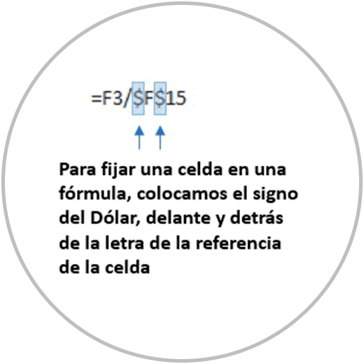
To fix a cell in a formula in Excel we are going to use the Dollar sign ($) ; We are going to place the $ sign before and after the letter of the cell reference that we want to set , inside the formula.
Steps to fix a cell or reference in a formula
- We are located in the cell where we want to make the Excel formula. We write the Excel formula, as we already know, starting with the “=” sign or with the “+” sign
- We type the formula, as we normally do, using our computer's keyboard or mouse to be able to include the cell references in the formula.
- When we finish making the formula, we edit it by placing the dollar sign. (which we will see on our keyboard) just before and after the letter of the cell reference that we want to set.
Error fixing a cell in a formula in Excel
It is very common, especially when we start learning Excel, to have errors when we try to fix a cell.
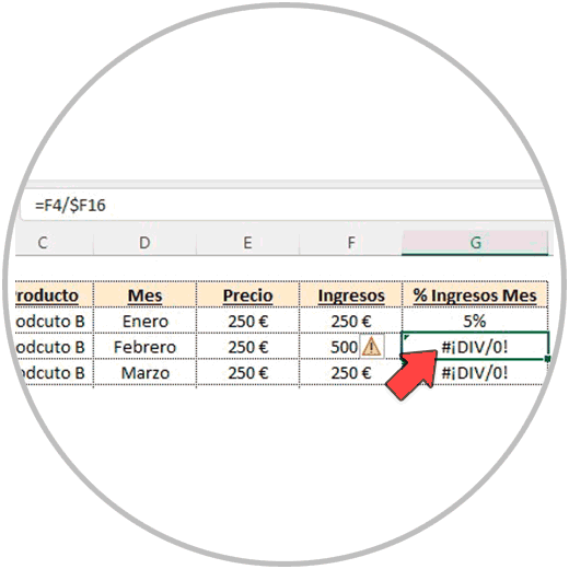
The reason when we want to fix a formula in Excel and receive an error instead, is mainly due to the wrong placement of the $ sign in the formula. It is very common to place the dollar sign in front of and after the cells. However, as we have explained above, the Dollar sign must be placed before and after the letter of the cell reference, as you can see in the image.
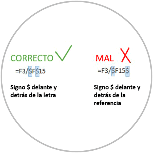
We must also check that the two dollar signs have been placed, that we do not need to place it before or after the letter.
When to Fix a cell in an Excel formula?
This situation of wanting to fix a cell in an Excel formula can occur when we want to create a formula and we want to drag the formula to other cells keeping one of the formula references constant. For example, when we are building a table and we want to add a column where we want to perform a calculation referenced to one of the totals.
Let's take a better look at how it works and how to fix a cell in a formula in Excel with an example, to see all the steps.
2 Example how to fix cells in Excel formulas
Let's imagine that we are building a data table where we have the sales made at the month level by product. We already have the income generated per month, and therefore we know the total income generated per year, which we have calculated with the sum function, which sums up the entire column.
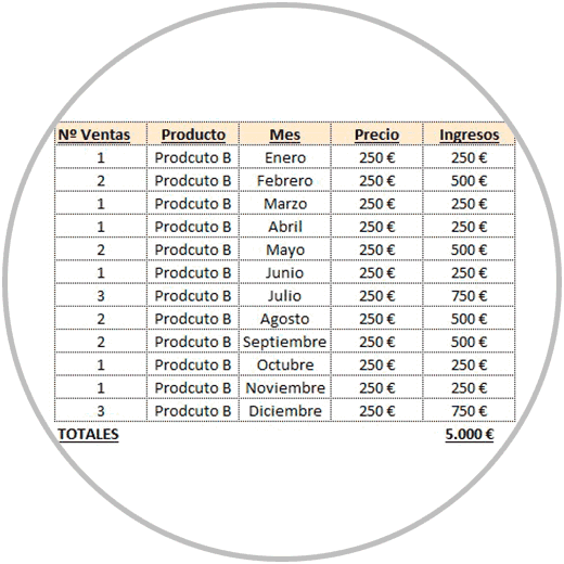
If we want to see what percentage of the total income we attribute to each month, we will have to perform an operation (in a new column) that involves the income that has been generated each month, and the total income generated in the year. The formula would be the following:
Monthly income/ Total year income
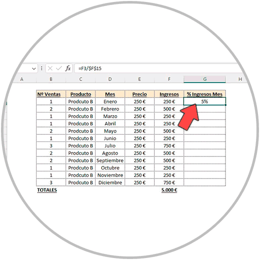
We are going to perform the calculation therefore in the first cell of the column, just below the header of the table.
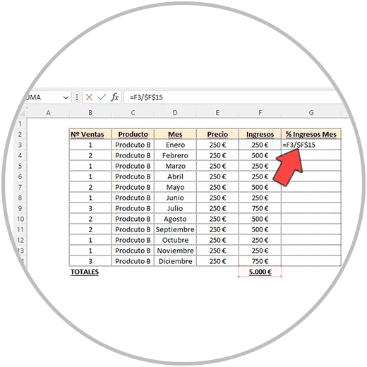
Now as we have explained to you, we are going to edit the formula and we are going to place the Dollar sign in the cell reference, just before and after the letter.
We will place the dollar sign before and after the letter of the cell that we want to leave as constant, which in the example will be cell “F15”.
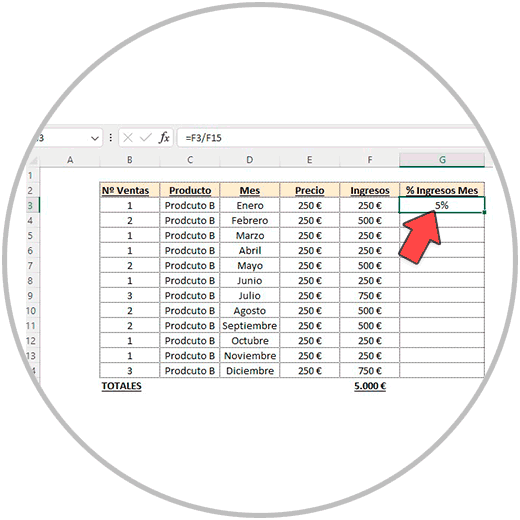
In cell "F15", there is the total income for the year, and it is therefore the cell that we are going to leave as constant, so that, in each month, the formula that is carried out is the income for the month, between the total of income for the year. This is how we will calculate the % of income for each month.
After carrying out the formula, we press the "Enter" key, and we see the result that we have obtained for the first month, which corresponds to the month of January.
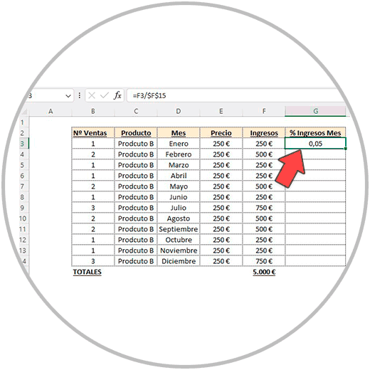
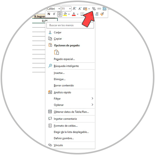
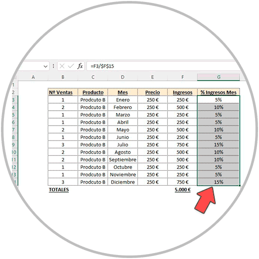
Now, before stretching the formula, we are going to change the format of the cell, clicking on the right button of the cell, and choosing in the window that the “percentage style” is displayed.
Now that the percentage format has been chosen, we are going to stretch the formula to the cells below to complete the table. Remember that, in order to be able to drag the formula, we place ourselves with a click on the cell that we want to “stretch”, and we will click on the little square that is in the lower right corner of the cell.
We then click on the small square in the lower right corner and without letting go, we drag to the last cell where we want to apply the formula. We release the click, and we will see the complete table with the % of income in each row, in each month.
Now we check that the calculation has been carried out correctly, and that cell "F15" is a constant in the formulas. We can move to any cell where we have applied the formula, and double click on the cell to see what references the formula has.
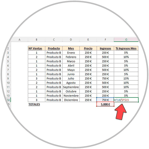
As we can see in the image, cell "F15", which is the total income generated throughout the year, has remained constant in all months.
Now we know that when we want to go faster in the construction of tables, we can use the Excel formulas, we can stretch the formulas, and we can also fix the references that we need in a cell when we want them to be kept as a constant.
In the examples, we have seen how to apply the Dollar symbol in the formula, before and after the letter of the reference that we want to set. We have seen simple examples that can be perfectly extrapolated to more complex formulas where we need to maintain a constant reference in the formula. One or more, because in longer formulas that involve more cells, we could similarly set more references within the same cell.
As always, and especially when we start working with Excel from the beginning, it is important that we check the work done, and that in this case, when we drag formulas to other cells, the calculations are carried out correctly, that the correct formula is applied in each cell. When we stretch formulas to other cells, we can check, as we have explained before in the example, that the last cell where the formula has been dragged is correct.