We explain how to extract data from a cell, using the “FIND” and EXTRACT functions, two very useful Excel resources when obtaining data from a text string. Learn how to use them easily, we explain it to you with examples..
When we are working on an Excel file, we encounter situations that invite or force us to obtain or extract a part of the information contained in one or more cells.
The reason or reasons that push us to have to obtain part of the information from a cell lies in the need to separate the information into cells in order to perform an analysis correctly . Thus, only in this way, we can treat and manipulate each information or data independently: We can make sums of columns, because they contain the same type of information, or perform a calculation, ratio or any other mathematical operation, such as taking an average, a value. maximum.
How could we add up the total sales of a company if we do not have this information organized in a column?, or How could we add up the sales of a company if this information is collected in a column that also contains text or Does it contain other types of aggregated or concatenated information? The secret is knowing how to separate the information, knowing how to disaggregate it and separate it into columns to be able to independently analyze the values. Thus, the sales of a company must be collected in one column, the income in another column, the expenses in another column, and so on..
Important
It is precisely for this reason that we must always, always,
always work in Excel in an orderly manner, in data tables; Tables that contain columns, and in each column a typology of information is collected .
Grouping information within a cell prevents us from being able to work easily with the information, it prevents us from being able to analyze it, it prevents us from performing mathematical operations with those cells and being able to use functions to analyze the information correctly.
As we already explained to you in how to separate text into columns, sometimes we find Excel sheets that do not have this rigor, either because they come from another source, from other people, or because we ourselves have not organized the data well; Data that for whatever reason does not have a correct organization, or contains grouped information, and it is we who have to work and analyze said information..
Whenever it is up to us, we will organize the information in tables, using the columns to classify the information, so that each column returns the same information for different records.
And if you need to group information within the same cell, remember that we must build our data table, with the same rigor, respecting the order, and working the information in columns. Thus, later, we can group or concatenate the data in another column, in a very simple way, as we already explained in how to concatenate data in Excel.
When we concatenate the information correctly, using the same separator, such as a comma, a period, or a space, separating the information later will be a simple task. The problem that we can often encounter is that we work with tables of data or information that we have not organized that do not have a common pattern in the separation of the information that a cell contains, or that simply that separator between the information in a cell does not exist and is therefore difficult to separate quickly or easily.
It is in these cases where we are going to have to use other techniques that allow us to achieve our objectives, which in this case would be having to extract part of the information from one or more cells.
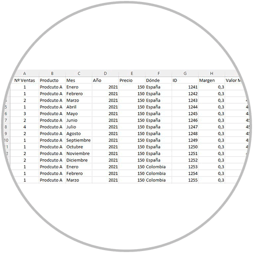
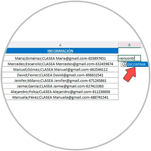
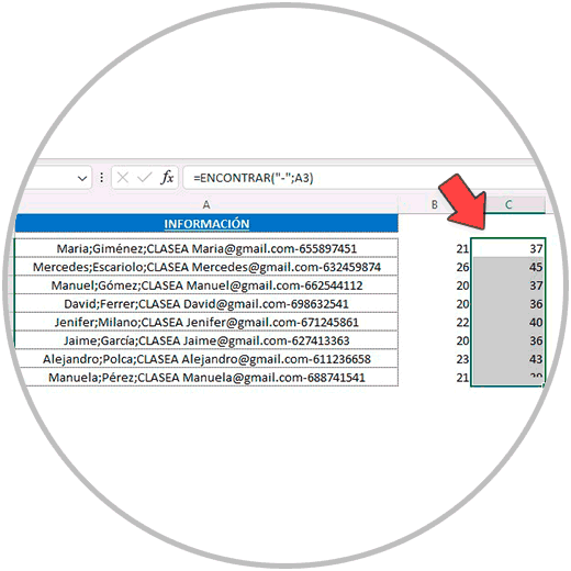
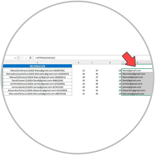
Let's see this explanation better with an example. In the image below, we can see a data table that contains information aggregated in the cells. If we look closely, within a cell, we can see how we have the information corresponding to the first and last name of several students, as well as the class to which they belong within the school. We can see your email and phone number. All this information is found within the same cell for each student.

In this example, the one we have seen in the image, how could we then extract, for example, only the email? The answer is by using two very useful functions: the “FIND” function and the “EXTRACT” function.
“FIND” and “EXTRACT” function in Excel: what they are for, and how they work
The “FIND” and “EXTRACT” functions are very useful in these cases where we want to extract specific information from a cell. We are going to explain to you what each of these functions provides, what they are for, and why they are useful for this same purpose: extracting information from a cell.
"FIND" function in Excel
The find function is used to find the position of a character, number or symbol within a text string. When we use the “FIND” function in a formula, the result of the formula returns a number; A number that determines the exact position of that character we are looking for, within the text string.
Thus, by using the find function, we could locate in each case the exact position of a character that is being used as a separator within a cell.
In the example that we have seen before, with the “FIND” function we can know what specific position the space has in each cell, and what position the hyphen (-) has.
These two elements in particular, the space and the middle dash, are the elements that separate each student's email, as we can see in the image below.

Steps to extract information from a cell
We are therefore going to create two new columns in our example, in order to determine the position of the space and the hyphen using the “FIND” function.
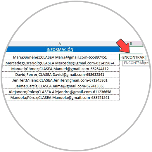
We therefore position ourselves to the right of the first row that has information, and we begin to write the name of the function, which as we already know is called “FIND”.
When we see that the Excel autocomplete shows us the “FIND” function, with the blue box, we double click (remember to double click on the name of the function).
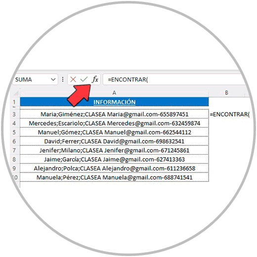
Now we see how it places the name of the function in the formula, opens the parenthesis and tells us what arguments of the formula or information the “FIND” function specifically needs.
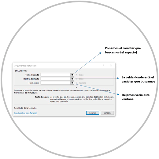
To finish completing this formula, we are going to use the “Formula Arguments” wizard. To open the wizard, we click on “Fx” , just to the left of where the formula bar is located, as in the image:
The wizard will then open, which helps us build the formula. Just by filling in the windows, the formula we need will be built. Look in the image below what information we must enter in each case, what information needs to be entered in each window.
Next, we continue with our example, and fill in the information that the wizard needs to be able to build the formula.
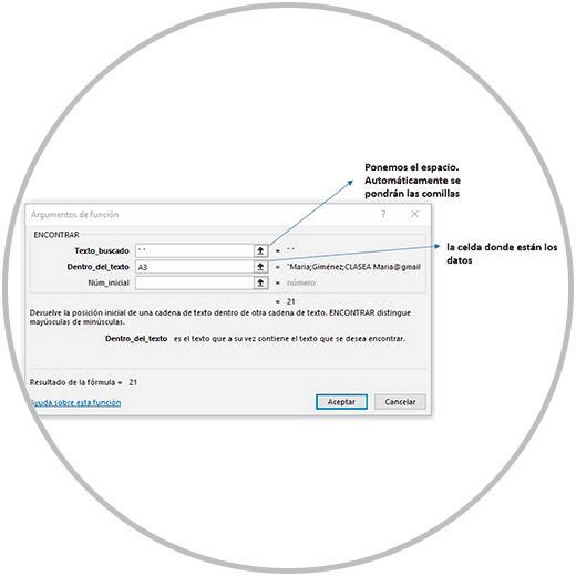
We click on “Accept”, and we will have the position of the space occupied by the first student's email.
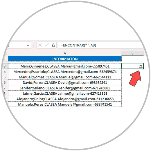
We extend the formula to the last row containing data, stretching the formula from the bottom right corner.

Once the position of the space has been calculated, we are going to perform the same operation to calculate the position of the middle dash (-), which is the first character that if you remember the cells had after the email.
We perform the same operation, in this case to obtain the position of the middle dash (-). To perform this operation we follow the same steps using the “formula arguments” wizard.
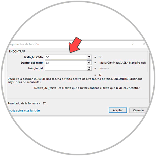
By clicking OK, we will now obtain the position of the middle dash. We stretch the formula to the last row to obtain the position of the middle dash of all students.
Now that we have the position of the elements that separate the email within the cells, we can move on to the second part of the process, which would be to use the “EXTRAE” function to obtain the email of each of the students.
As we have seen, the “FIND” function is very useful for determining the position of a character, but it is even more so in combination with other functions that need to determine the position of that character in order to later extract information.
This is the case of the “EXTRAE” function, a function that allows us to choose part of a text string, but that works only if:
- We have the exact information of the position occupied by the text that we want to extract within the string.
- We must also know the exact number of characters in the text we want to extract. In the example, we have to first find out how many characters each email has.
Extract Function in Excel
The extract function helps us obtain several characters from a cell but only if we have the “coordinates” of the text, and the length of the text.
In this sense, the find function, as explained first, is crucial to being able to know the position of a character within a formula. Determining the position is especially useful when, for example, we want to extract part of the content in several cells that do not have the same number of characters, as is the example case we are working on.
If we notice, the position of each student's email within their cell is a different position.
Let's see what coordinates the “EXTRAE” function now needs to be able to obtain the text we want, which in the example if we remember was the email of each student.
- On the one hand, we need the initial position of the email. Position that we already have calculated thanks to the find function, which we used before to determine the position of the space that is just in front of the email information.
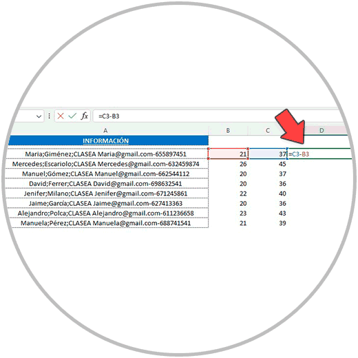
- On the other hand, we need to know how many characters we need to extract in each case. As each email has a different length, it would be difficult to carry out. However, we have very valuable information, which is the space occupied by the middle dash (character found after the email in each case).
- If we subtract the position of the middle dash from the position of the space, we will therefore obtain the number of characters that each email has.
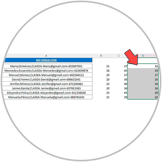
In a new column, we then calculate the No. of characters that each email occupies, for each student. To perform this operation, we are going to subtract the position of the space from the position of the script, as in the image.
Then we drag the formula to the rest of the rows to be able to have the number of characters in each student's email.
Now that we have this information, we already have all the data to be able to use the “EXTRAE” function.
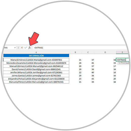
In another column, to the right, as we write the “=” sign, and we begin to write the name of the function, which is called as we have said “EXTRAE”.
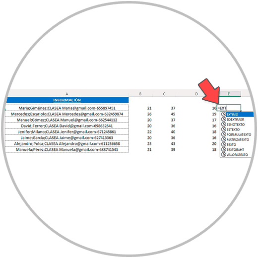
We click in the blue window, on the name of the function, so that it places the beginning of the formula correctly, and then we click on “ FX ”, to the left of the formula bar, to open the wizard “ function arguments”.
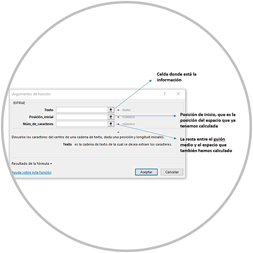
Now we are going to fill in the information required by the use of the “EXTRAE” function as follows:
- In text we select the cell where the data is
- In Initial Position, it is the position of the space that we have calculated before
- The number of characters is the value of the subtraction that we just performed, where we subtracted the position of the middle dash and the position of the space, to obtain exactly the number of characters in each email
Therefore, we fill in the information requested by the assistant.
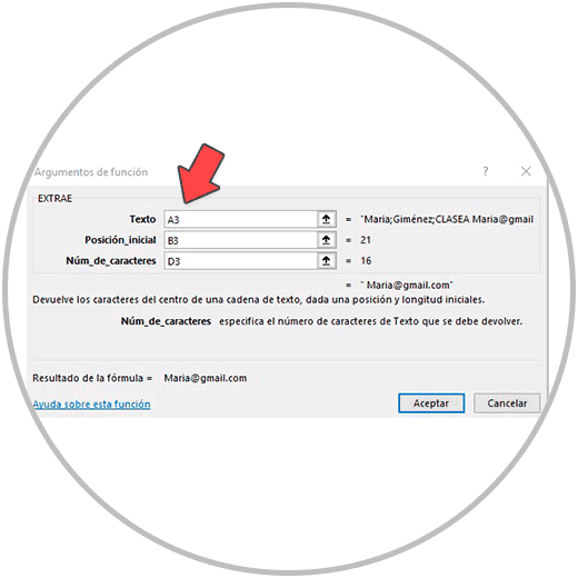
By clicking OK, we see how we have finally managed to extract the first email.
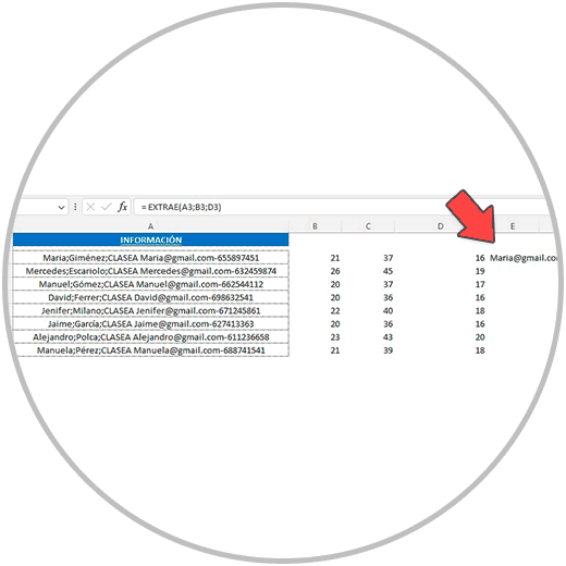
We stretch the formula to the row that contains the information of the last student, and we have already managed to extract the email of the rest of the students.
In this way, we have learned two new resources in Excel that give us more freedom when it comes to working more quickly, and better solve situations in which, for some reason, we are forced to have to extract part of the information we contains one cell.
Remember that the use of the formula assistant, which we call “Formula Arguments”, is a very practical resource that makes our task easier when constructing the formulas; Thus, we do not have to be aware of the use of quotes, parentheses, or the general structure of the formula.
Knowing, as they say, takes up no space, and we consider it very important in learning Excel that you also know how to build formulas without the wizard; But if necessary, and especially at the beginning, when we do not know the structure of certain functions, it can be tremendously useful.