Microsoft has developed Excel as an application through which we have a series of tools such as functions , formulas, dynamic tables and more to work with data management. This is something that gives many people a headache , but with Excel it will be something really simple no matter what type of data we work there..
We know that when some users hear "Excel" they are in crisis because the possibilities of work are really wide, but when we become familiar with their surroundings and with their possibilities we will notice that the results are more than satisfactory since the data can be represented in a way much more global to highlight each of the expected results.
One of the most common ways we can represent data in Excel is to display or highlight the results using colors . With this function we can configure that if a value is in a certain range its cell has a color and if that value changes another color is applied. This will dynamically help the results are much more visible and understandable by other users. It also gives a more professional and worked to the presentation of the results, is it what we want? Well, TechnoWikis will explain how we can carry out this task completely in Excel..
To stay up to date, remember to subscribe to our YouTube channel! SUBSCRIBE
1. How to make an Excel 2019, 2016 cell change the color automatically
Step 1
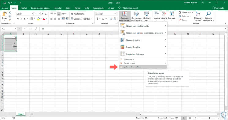
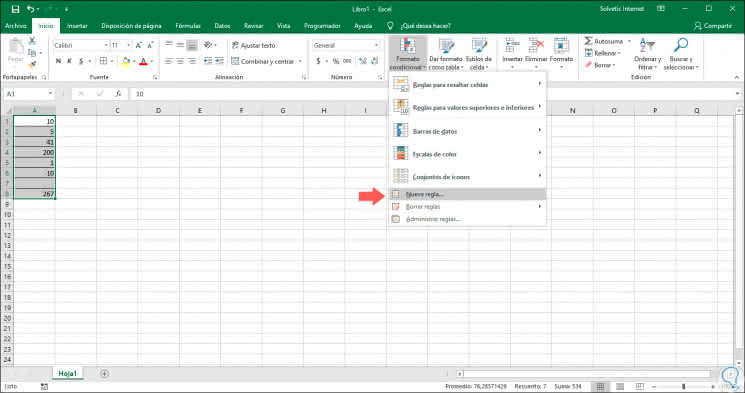
To carry out this task in a practical way we will use rules, in this case we will select a range of cells where the values ​​are, this also applies to a single cell if we want, once the range is selected we will go to the menu "Start" and in the group "Styles" we click on the option "Conditional format" and in the list we will select the option "Manage rules":
Step 2
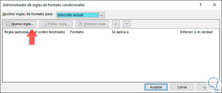
The following wizard will be displayed:
Step 3
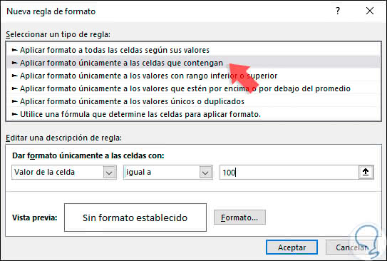
There we click on the button "New rule" and in the next window we select the rule called "Apply format only to the cells that contain":
Step 4
We see in the section "Edit a rule description" where we can apply the following conditions:
- Set the Cell Value field.
- Assign the type of variable to use, the options are: between, not between, equal to, not equal to, greater than, less than, greater than or equal to or less than or equal to, this will be defined based on the values ​​in the cells and according to the expected result.
- We will assign the value to evaluate.
Step 5
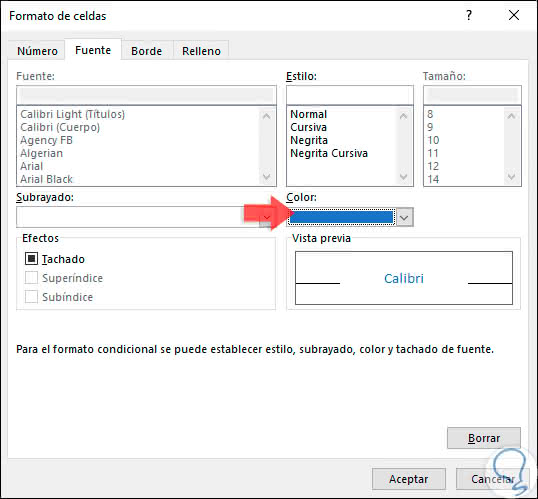
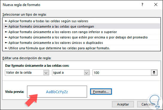
In this case we have determined that the format will be applied if the value in the cell is equal to 100, now, to assign the color of the cell we click on the "Format" button and on the "Source" tab and in the field " Color "we will assign the desired color to apply in the cell that meets that condition:
Step 6
We click on OK and we can see a preview of how the style would look in the cell:
Step 7
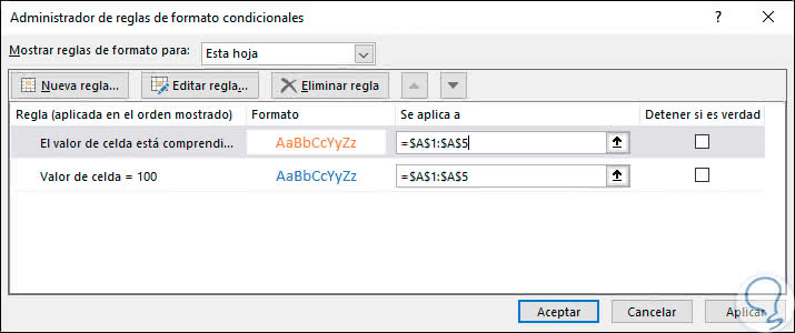
We click on OK and it will be possible to manage the rule that we have created:
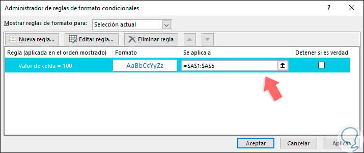
Step 8
There it will be possible to add more rules with new conditions, edit the current rule or delete it, if we only use this rule click on Apply and then OK to see the results in the Microsoft Excel sheet:
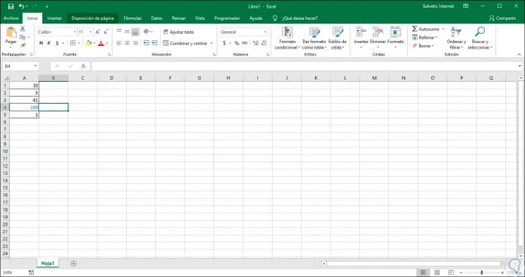
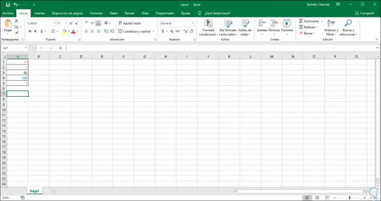
Step 9
As we can see, only the number that fulfills the condition has been modified with the selected color.
Now, as we are professionals in what we do, we probably want to add more rules with different conditions, in this case we go back to the Start menu, group "Styles" and in "Conditional Format" and select "Manage rules":
Step 10
There we click on the button "New rule" and again select the option "Apply format only to the cells that contain", in this case we will edit the values ​​between 1 and 20 with orange:

Step 11
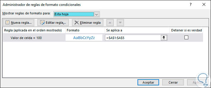
Click on OK and we will see the new rule added:
Step 12
Click on Apply and Accept and we will see that the rules are applied to the range based on the selection of both parameters and colors that we have defined:
2. How to make an Excel cell 2019, 2016 not change the color automatically
Microsoft Excel allows us to define some key points about the assignment of rules, these are:
- We can change the background color of the cells according to the value dynamically which will change when the value of the cell changes.
- It will be possible to change the color of special cells such as cells with blank spaces, with errors or with formulas.
- We can also change the color of a cell based on the current value statically, with this parameter, the color will not change so the value of the cell is modified.
The method that TechnoWikis has explained to you before is the dynamic method because if we edit any of the values ​​it will be evaluated based on the defined rules. Now, if we want to use the static method, that is, the color of the cell does not change even if the cell values ​​do.
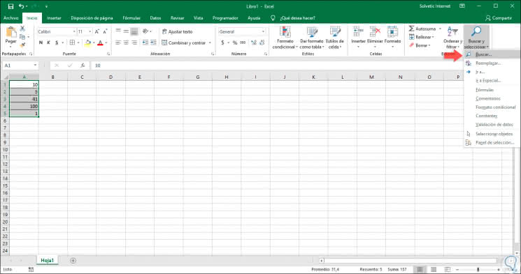
Step 1
To do this, we go to the Start menu and in the Edition group we click on Search and select and in the options we choose "Search":
Step 2
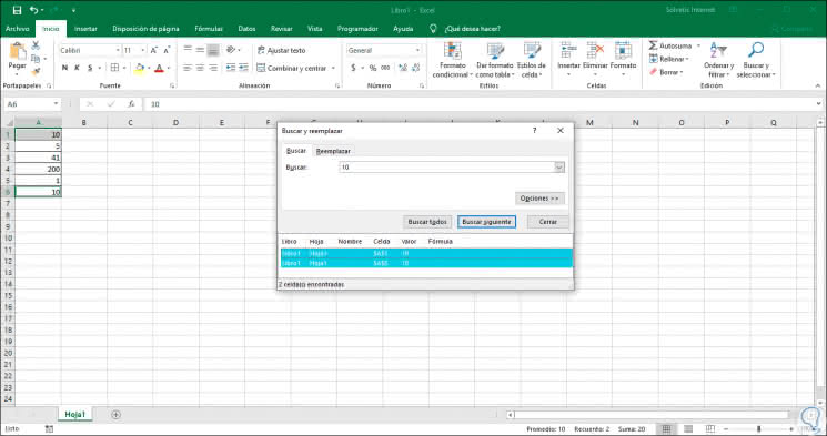
In the window that will be displayed, enter the desired number in the "Search" field:
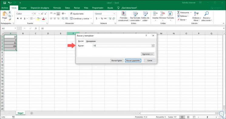
Step 3
We will click on the "Search for all" button and at the bottom we will find the row in which the desired value is:
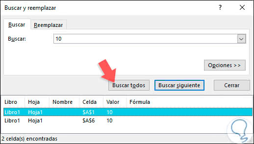
Step 4
Proceed to select all the results with the "Ctrl + A" keys and note that the cells are selected in the range where they are currently:
Step 5
Click on the "Close" button to exit the wizard, and in this way it will be possible to select all the cells with the required value through the Search All function in Microsoft Excel.
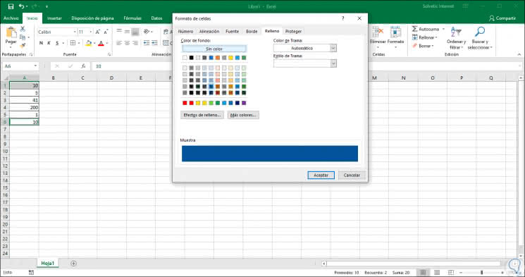
With our selected cells we will proceed with the use of the format to be applied in these, for this after closing the "Search all" wizard we can verify that the cells with the searched value will remain selected. Now we will use the following keys to access the "Format of cells" and in the "Fill" tab we select the desired color:
+ 1 Ctrl + 1
Note
To access this option it will also be possible in the Start / group Cells route, option Format / Format of cells.
Step 6
Click on "OK" and the cells with these searched values ​​will have the desired filling:
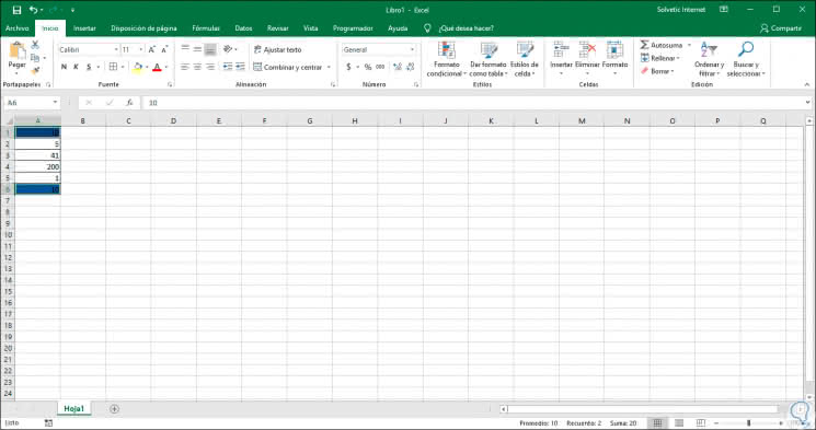
Step 7
Now we can change the value of the cell without the color being modified. On the other hand, if our objective is to edit special cells, such as blank cells or cells that have formulas, in this case we select the range to use, then we will go to the Start menu, the Styles group and there we click on "Conditional format" to select the option "New rule":
Step 8
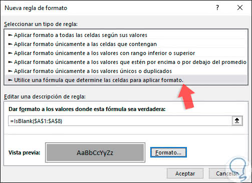
In the expanded window we will select the rule called "Use a formula that determines the cells to apply format" and in the lower field we will enter any of the following options:
= IsBlank ()
This applies if we want to change the background color of the blank cells.
= IsError ()
This option allows you to change the background color of the cells in which formulas with errors are found.
Step 9
In the lower part we will define, as we have seen, the color to apply in the format and it is vital to clarify that the range must be after the selected formula:
Step 10
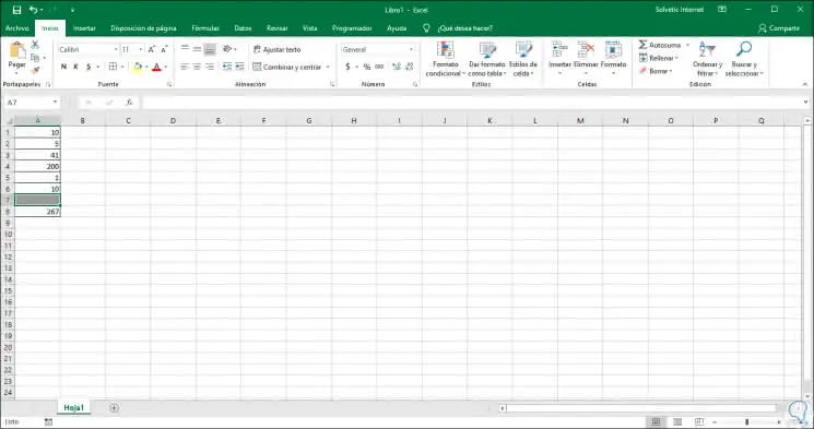
Click on "OK" and we will see that the color has been applied to the defined cell, in this case a blank cell:
We have learned to put aside the fear that thousands have to Microsoft Excel and to understand how with a few steps, all of them simple, we can achieve comprehensive and complete results that facilitate not only the reading of information but also give us options for a professional and dynamic presentation..