One of the great advantages of Microsoft Excel 2019 is its ability to process large amounts of data in a simplified manner thanks to its integrated functions and formulas which, once correctly configured, will give us the expected results with few steps, thus helping to save time and resources of each user that manages Excel 2019. Within all the set of functions incorporated in Microsoft Excel 2019 we find a special category that are the logical functions and within them we find two special ones that are the functions Y and YES..
The Y function gives us the possibility to determine if all the conditions of a cell are TRUE and the SI function gives us the possibility of carrying out logical comparisons between a value and the result that we hope will be returned.
1. How to use the Y function in Excel 2019
When using the AND function, it will return TRUE if all the arguments in the cell are evaluated in this TRUE state, otherwise it will return FALSE if one or more of the arguments that are in the cell are taken as FALSE.
Its usage syntax is:
Y (logical_value1, [logical_value2]
The arguments to use are:
Logical_value1
It is a mandatory value and represents the initial condition that has to be evaluated and whose status can be TRUE or FALSE.
Logical_value2
These are optional values ​​that can also be in a TRUE or FALSE state and with the AND function we can use up to 255 conditions.
To take into account when we use this function:
- If there are no logical values ​​in the range, the Y function will lead to the error # VALUE!
- In case we have empty text or cells, these values ​​will not be evaluated by the Y function
Using the Y function in Excel 2019
Now TechnoWikis will explain in a practical way how to make use of this function AND in Microsoft Excel 2019.
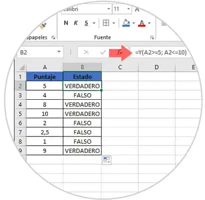
For this case we have a series of data (score) and we will use the SI function to determine that all values ​​greater than or equal to 5 but less than or equal to 10 will obtain a TRUE value, otherwise the result will be FALSE, for this we execute the next:
= Y (A2> = 5; A2 <= 10)
2 How to use the IF function in Excel 2019
This function is one of the most used and practical in Excel 2019 and its mission is to return a value if one condition is true and another if the evaluated condition is false.
Its usage syntax is the following:
YES (logical_test; value_if_true; [value_if_false])
The arguments used are:
logical_test
It is a necessary value since it is the value that has to be evaluated
value_if_true
Another mandatory value since this refers to the result that the IF function will return if the result of the analysis is TRUE.
value_if_false
It is an optional value and indicates the result that IS generated if the condition is FALSE.
Use of the SI function with ranges of values ​​in Excel 2019
Recall that the function is in the ability to evaluate the condition of a logical test through multiple parameters to obtain the desired result.
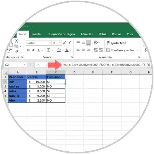
For this case we take as an example a group of sellers and their respective sales, if the sales exceed a specific range they are entitled to commission, otherwise no, the formula to be used will be the following:
= YES (Y (B2> = 100; B2 <= 5000); "NO"; YES (Y (B2> 5000; B2 <20000); "YES"))
Thus, sellers whose sales are greater than 100 but less than or equal to 5000 will not commission, from 5001 to 20,000 if they achieve commission:
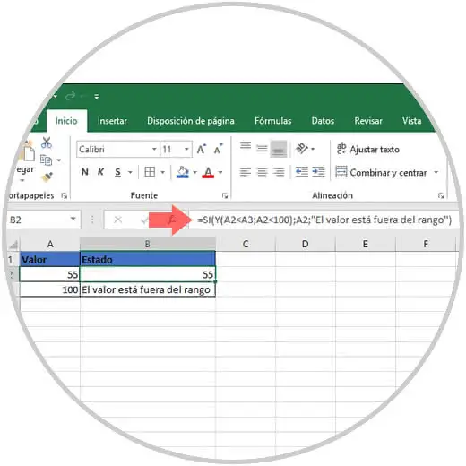
This is achieved thanks to the nested SI function, but it is also possible that we want to display a text in the result, for example, we will execute the following formula:
= YES (Y (A2 <A3; A2 <100); A2; "The value is out of range")
There, we will see the value of cell A2 if the value is less than A3 and if it is less than 100, on the contrary the message "The value is out of range" will be displayed:
3. How to create a range of variable numbers in Excel 2019
Excel 2019 is a special application for the management of numerical data thanks to its functions. In many tasks we are presented with ranges of different numbers and we must define whether these belong to a specific area or not, for example we can define segments such as:
- Greater than or equal to 5 / Less than or equal to 10
- Greater than or equal to 15 / Less than or equal to 20
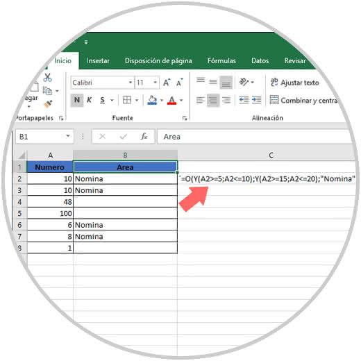
If we use these ranges, the formula to be implemented will be the following:
= Y (A2> = 5; A2 <= 10) Y (A2> = 15; A2 <= 20)
With this formula an individual task is created for each cell, to create a global formula that affects all the cells where the data is found, we must add the O function like this:
= O (Y (A2> = 5; A2 <= 10); Y (A2> = 15; A2 <= 20); "Nomina")
The results that are not in that range will have their empty cell in the execution of the formula:
4. How to create a dynamic range in Microsoft Excel 2019
Microsoft Excel 2019 gives us the opportunity to have an assigned range which can be extended to include new information at a given time. Recall that a range of cells in Microsoft Excel indicates a group of adjacent cells on which we can perform various tasks such as applying formulas from another cell, but if these add or decrease the information of these cells instead of updating the formula individually the Dynamic range will do it for us.
Step 1
Microsoft Excel integrates the dynamic range function as a method in which a range of cells will be adjusted automatically based on the fact that this range is edited with the modification of its data.
When a dynamic range is implemented in Microsoft Excel, two functions are used, which are:
The DESREF function has the task of returning a reference to a range which is a representation of a number of rows and columns. The reference generated by DESREF can be represented by a cell or a range of cells and we are able to define the number of rows and the number of columns to be returned.
Its syntax is the following:
DESREF (ref, rows, columns, [height], [width])
Step 2
The arguments to use with DESREF are:
Reference
It is a necessary value since it is the reference on which the deviation will be based and this can refer to a cell or a range of adjacent cells, if not, we will observe the error # VALUE !.
Rows
It is another mandatory value because there we will indicate the number of rows, up or down, in which the reference of the upper left cell will be used.
Columns
It is a mandatory value since it indicates the number of columns, to the right or left, in which the reference of the upper left cell of the result will be made.
High
It is optional since there we can indicate the height of the rows
Width
Another optional value where reference will be made to the width of the columns.
The CONTARA function of Excel 2019 is a statistical function whose purpose is to analyze the range of the selected cells and count the number of cells that are not empty to display the results..
Its usage syntax is:
COUNTA (value1, [value2])
Step 3
His arguments are:
Value1
Indicate the first cell or range from where we are going to count.
Value2
They are additional cells or ranges that we can add to the argument, CONTARA supports up to 255 conditions.
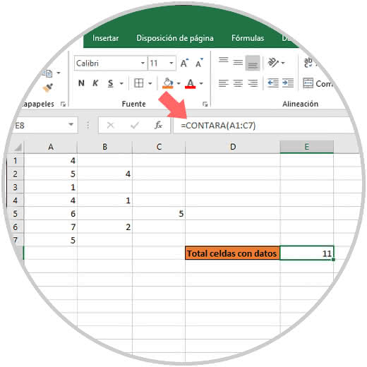
As an example, let's execute the following:
= COUNTA (A1: C7)
There we will count the cells that have some value in that range:
Step 4
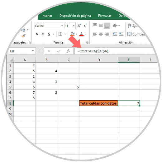
Another option to obtain the data of the cells with some value, is to add by columns, for example to see the cells with data in column A we execute:
= COUNTA ($ A: $ A)
Step 5
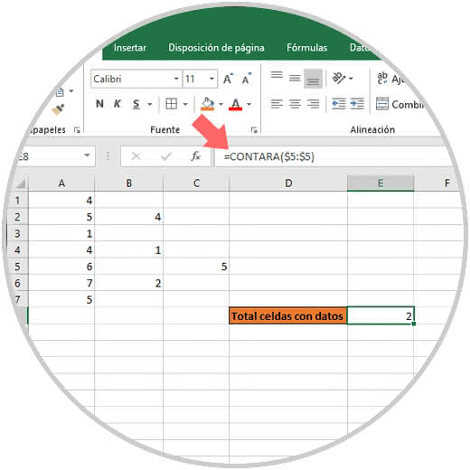
Another useful option is to identify how many cells have data in a row, for example, to know the cells with some value in row 5 we execute:
= COUNTA ($ 5: $ 5)
5. How to combine the functions COUNTA and DESREF in Excel 2019
Now we are going to use the combination of both functions to create our dynamic range, this process is composed of several steps that TechnoWikis will explain carefully:
Step 1
First we will indicate the initial cell from where the range to analyze will start:
= DESREF ($ A $ 1,
Following this, we will define how the formula will move from the initial cell, this value can be zero if no special route has been defined:
DESREF ($ A $ 1, 0, 0,
Step 2
Now we are going to add the COUNTA function in order to determine the number of rows and columns of the range, in order to determine the number of rows we enter $ A: $ A:
= DESREF ($ A $ 1, 0, 0, COUNTA ($ A: $ A),
For the rows we enter $ 1: $ 1:
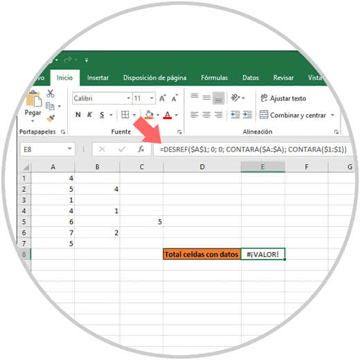
= DESREF ($ A $ 1; 0; 0; COUNTS ($ A: $ A); COUNTS ($ 1: $ 1))
When executing this formula we will see the following error:
Step 3
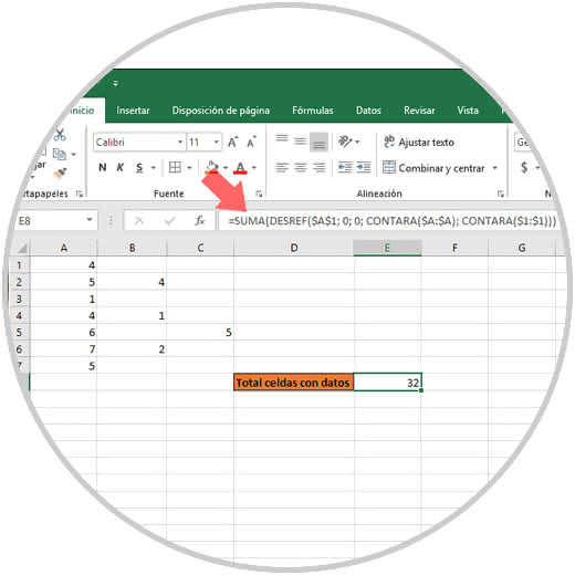
This is because the formula returns a reference but not a value, for its correction, we will add the SUM function at the beginning so that Microsoft Excel 2019 adds the values ​​returned by the range defined with the function DESREF:
= SUM (DESREF ($ A $ 1; 0; 0; COUNTS ($ A: $ A); COUNTS ($ 1: $ 1)))
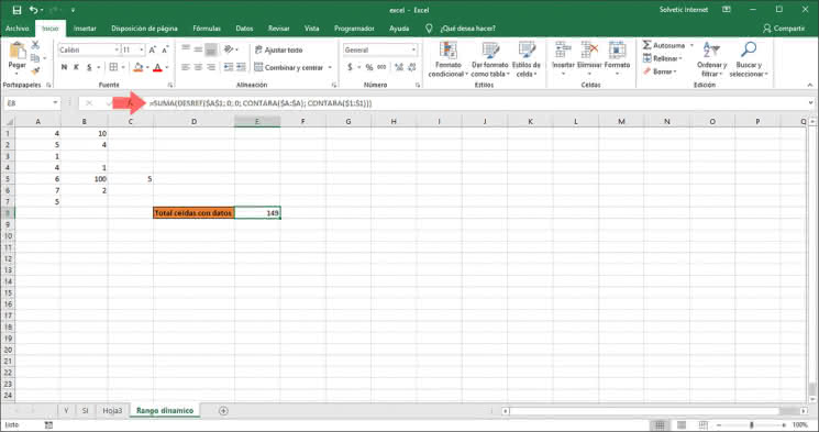
Step 4
Now, we enter new values ​​in cells B1 and B5 and we can notice that the result of the formula is automatically affected:
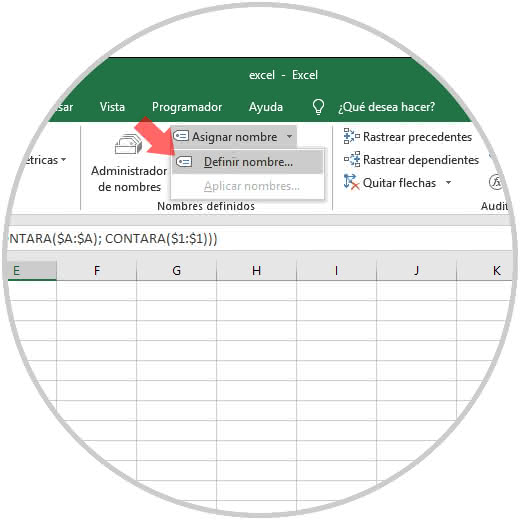
Step 5
We may want to assign a name to the dynamic range created for better administration, for this action, we must go to the Formulas menu and in the Defined names group we click on the Assign names option and there we select the Define name option:
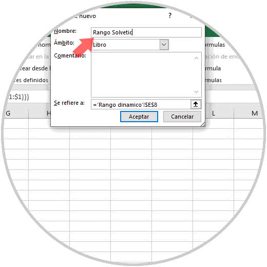
Step 6
In the pop-up window we will assign the desired name. Click OK to apply the changes.
We can see how the use of functions in Excel drastically simplify the execution of multiple tasks which in turn is reflected in time improvements and better control over the data to be used.