Data is the fundamental basis when we work in Microsoft Excel 2019 since without them it would be impossible to make formulas, functions, tables or any Excel integrated tool for the generation of optimal results. That is why a correct administration of this data will help us to have precise control over the result we want to obtain and, without any doubt, this will help to execute in a sure way the formulas that are necessary..
When managing large quantities or volumes of data, something natural in Microsoft Excel 2019, it is ideal to keep a precise order of the information stored there. This not only helps to improve the visual impact of the results, but it will also be a source of confidence when it comes to highlighting functions. Disordered or inconsistent data bring about bad administration , as well as an incorrect interpretation of the desired results.
For this reason, the new version 2019 of Microsoft Excel integrates a series of practical options to manage the order of the data and especially when we must organize these in an alphabetical way and therefore TechnoWikis will explain how to achieve this in a simple but effective way in Excel 2019 and thus have the possibility of better managing the data..
To stay up to date, remember to subscribe to our YouTube channel! SUBSCRIBE
1. How to sort alphabetically an entire active sheet in Excel 2019
Microsoft Excel 2019 gives us the possibility to organize all the data entered either by selecting only a range of cells or the entire active sheet.
Step 1
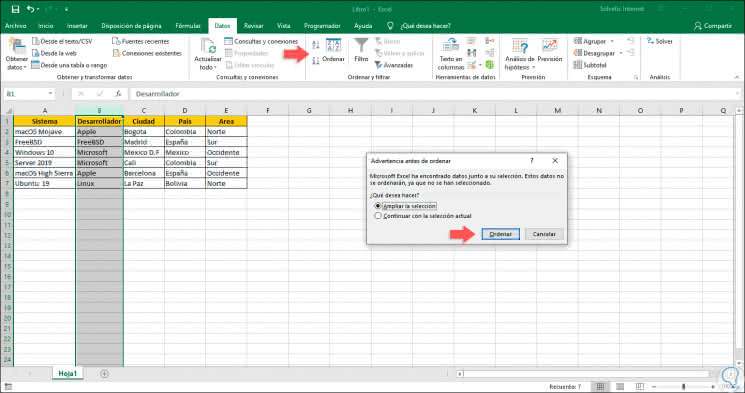
If we want to order the entire sheet, we just need to select the entire desired column and it is important to clarify that Excel 2019 gives us the option to sort the data either in ascending or descending order. For this we go to the "Data" menu and in the "Sort and filter" group we select some of the available options, either Ascending or Descending, in this case of a total sheet, the following message will be displayed:
Step 2
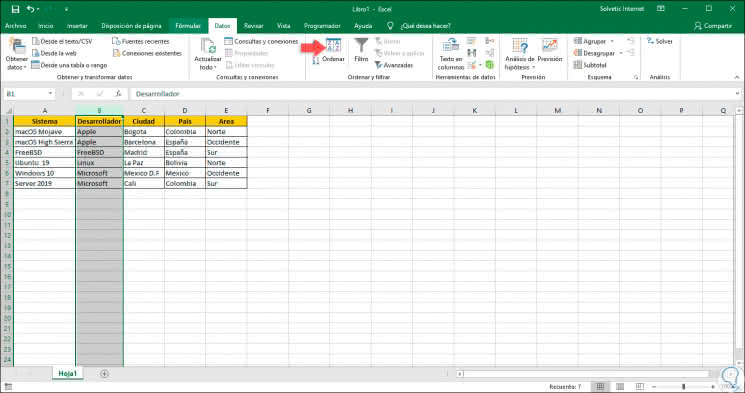
There we select the option "Expand the selection" and we will see that the data is sorted by the selected column:
Step 3
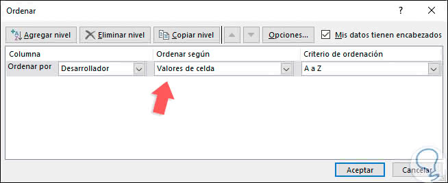
Another one of the integrated options of Microsoft Excel 2019 for the ordering of the data is to apply a series of filters based on the columns available in the sheet. For this method we select some of the columns with data and in the "Sort and filter" group we click on the "Sort" button and the following window will be displayed:
Step 4
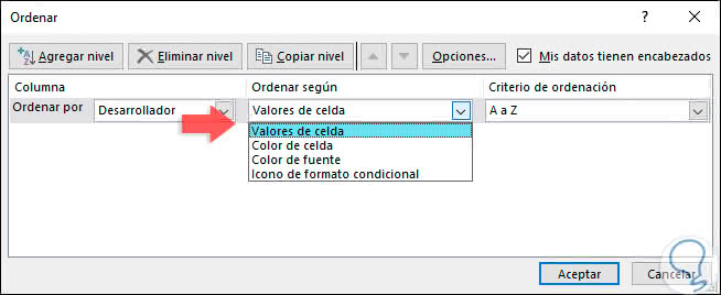
In this case, the first column defined is the one we have selected, there in the "Sort according to" field it will be possible to apply a series of filters such as:
Note
In the field "Sort order", you will define whether the data must be sorted in ascending or descending order.
2. How to sort alphabetically an entire active sheet with several criteria in Excel 2019
Excel 2019 has the possibility of applying a series of personal values ​​to the way the data has to be ordered, this helps to apply a series of filters on the columns to be sorted.
Step 1
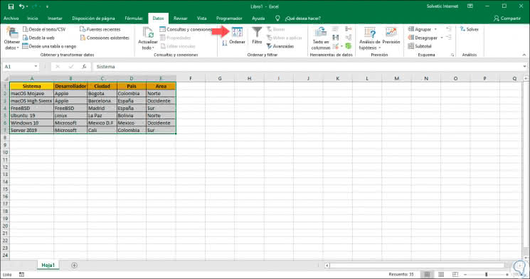
To achieve this, we select the entire range of cells where the data is located first:
Step 2
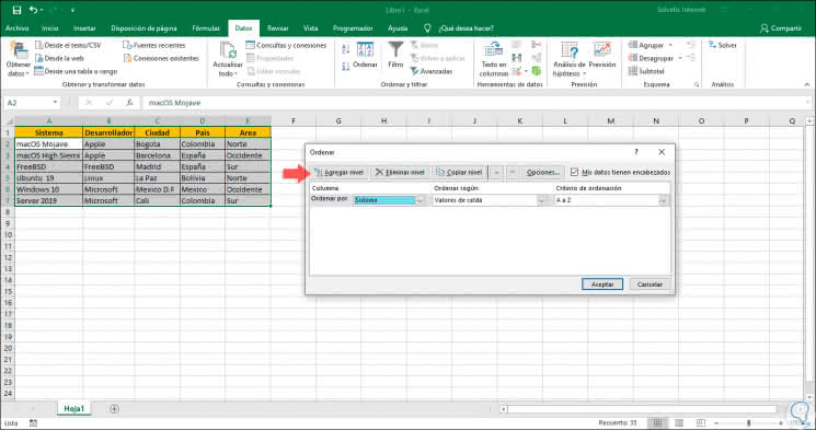
Now, from the "Data" menu, group "Sort and filter" we click on the "Sort" button:
Step 3
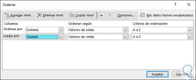
Note that in this opportunity the first column displayed will be column A, there we can define the desired organizational criteria. If we want to add another organization parameter for another column, we click on the "Add level" button and in the new field we will enter the column in which the following level of organization is to be applied:
Step 4
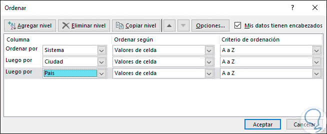
We can add more levels as we consider it necessary to sort the data in Microsoft Excel 2019:
Step 5
Click on "Accept" and automatically defined columns will be sorted based on the criteria we have defined previously:
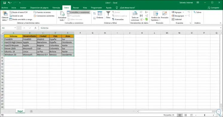
3. How to sort the data in Microsoft Excel 2019 according to the type in Excel 2019
Excel 2019 integrates different options that give us the possibility to organize the data according to the content or the type of these, we will see some examples of how Excel 2019 applies these filters in an integral way.
Sort the data by date
The date values ​​are one of the most common data when we work in Excel 209 and therefore they are one of the most delicate due to their level of syntax.
For this case we have the following information:
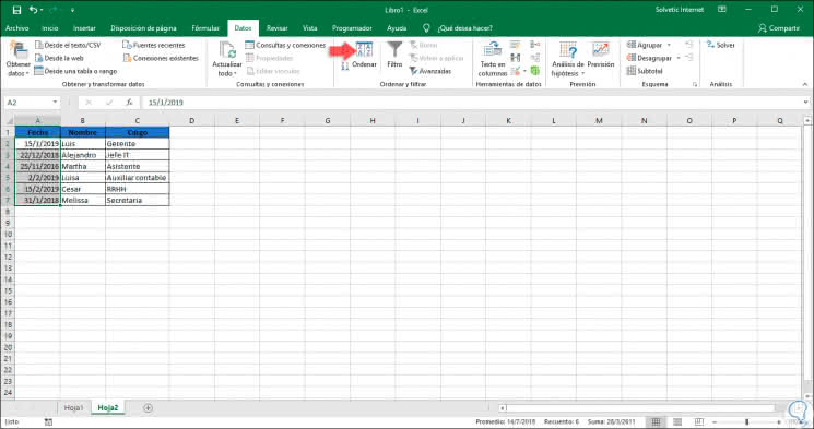
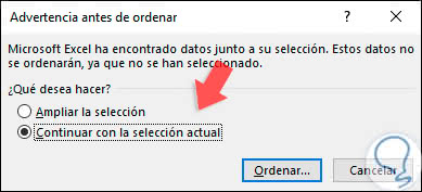
There we will select the rank of the column where the date values ​​are and proceed to go to the "Data" menu, group "Sort and filter" to click on the "Sort" option. The following message will be displayed where we select the option "Continue with the current selection":
Click on "Sort" and in the pop-up window there will be by default the column Date and note the different options integrated in Excel 2019:
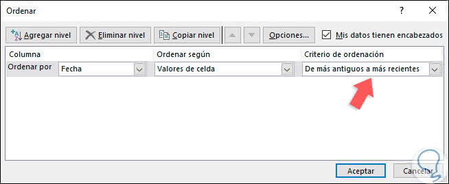
In the field "Sort order", in the case of dates, we have options such as:
- From oldest to most recent
- From most recent to oldest
In this case we select the option "From most recent to oldest", click on OK and this will be the result displayed:
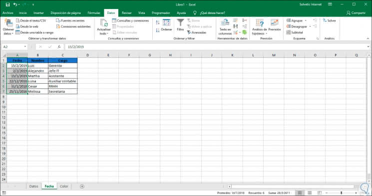
Something important to keep in mind is that if we select the option "Continue with the current selection" the filter will only be applied to the selected column or range. If we want the ordering to affect all the data we must select the option "Expand the selection" and we will see that the result is different:

Sort data by cell color
This is a practical option of Microsoft Excel 2019 since it will be possible to organize the data taking criteria such as the cell's fill color or the font color, we have the following information:
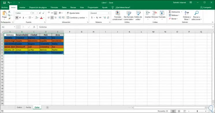
We select the data range and go to the menu "Data / Sort and filter" and there we click on the "Sort" option and in the displayed window we will apply the following configuration:
- Cell in which the filter is to be applied.
- In the "Sort by" field we can select the options "Font color or Cell color" as the case may be (in this case Cell color).
- We select the color by which the filter will be applied.
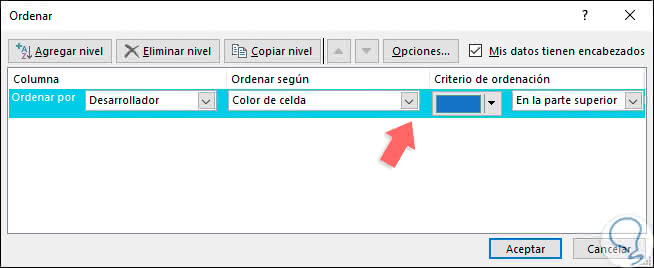
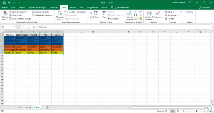
Note that an option is added and it is the location of the order which can be in the upper part or in the lower part. Click OK and this will be the result obtained by cell color:
4. How to sort the data in a personalized way in Microsoft Excel 2019
This option gives us the opportunity to create a personal filter according to the criteria we consider relevant for the data to be worked on.
Step 1
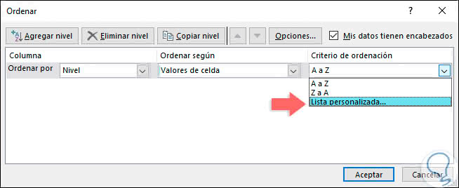
To use this method, we will select some of the cells where the data is and click on the "Sort" button located in the "Sort and filter" group of the "Data" menu and in the pop-up window we will select the column in which we have to apply the order and in the field "Sort order" we select the option "Custom list":
Step 2
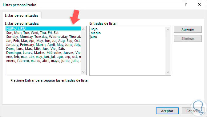
The following window will be displayed where we will enter the custom values ​​in the column "List entries":
Step 3
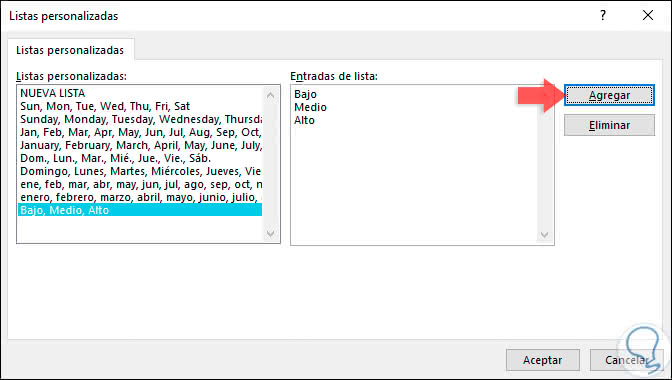
Click on the "Add" button and we will see these values ​​in list format in the "Custom lists" section:
Step 4
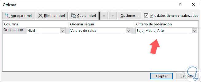
Click OK and now in the Sort Criteria field verify that this directly created option has been added:
Step 5
Press OK again and the data will be organized based on this criterion:
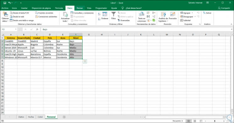
We see that the options to sort the data in Microsoft Excel are varied and complete according to the current need of each one of us, but each of them gives us the option to organize the information with a series of own criteria that will undoubtedly generate the best results based on the type of data recorded..