With an Excel table with a lot of data, it quickly becomes confusing. And confusion can just as quickly lead to errors. In order to be able to correct errors quickly, there is the IFERROR function in Excel. In the following article, we will explain how you can use this optimally.
Here you will find more Excel tips on the subject of target search, data verification and actual formulas.
How is the IFERROR function structured in Excel?
The IFERROR function in Excel is used to check your data in the table. A value to be checked is specified for this purpose. If one of the following errors occurs, the function spits out one of the following error messages: # N / a, #Value !, #ref !, # DIV / 0 !, #Num !, #Name? or #NULL !. The message takes place via a notification text that you can define yourself. If there is no error, you will be shown the result of the corresponding data instead..
The formula for the function is structured as follows:
=WENNFEHLER(Wert;Wert_falls_Fehler)
So the formula for the IFERROR function has two arguments:
Value : Here it must be specified what should be checked for an error. For example, you can specify cells that contain an invoice or represent the result of an invoice. You can also insert an invoice (with cell references) as a value yourself.
Value_falls_Error : Here you enter what should be displayed if an error is found. This can be, for example, "error in the calculation" or simply "error". The function then shows you this printout when an error has been detected. Please note : You can enter numbers without quotation marks in "Wert_falls_Fehler". However, you must put quotation marks in the formula for words or combinations of letters. In the following we show you two examples:
Example of an IFERROR formula
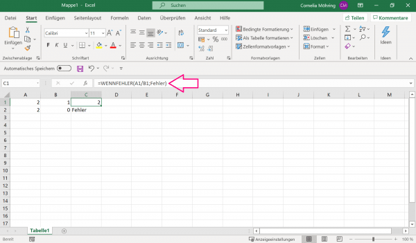
example 1
=WENNFEHLER(A1/B1;"Fehler")
 Here cell A1 with the value 2 has been divided by cell B1 with the value 1. The result is 2 and is therefore not incorrect. So the correct result is shown in cell C1.
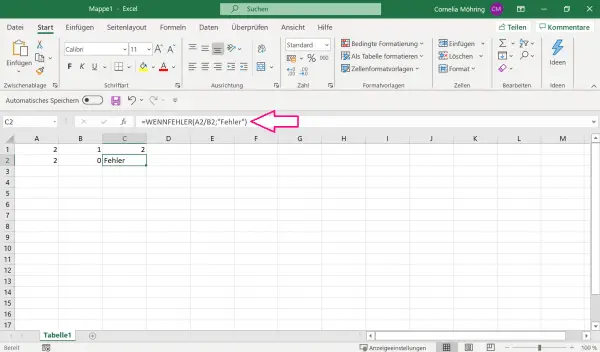
 Example 2
=WENNFEHLER(A2/B2;"Fehler")
 In this example, the value of the A column is again divided by the value of the B column. However, this time A2 with value 2 is to be divided by B2 with value 0. It cannot be divided by 0, which is why the set message "Error" is output in cell C2.