Formulas in Excel are a necessary resource when we work with data sheets in order to obtain calculation results and perform some operations. Through a formula, we can obtain results that are very valuable to be able to analyze the information and make decisions. In many cases, as we will see, calculations are necessary to be able to objectively analyze the data..
For example, what use would it be for us to analyze and compare the sales results of a company with the sales data of previous years, if we do not know the total sales made per year?
In this case, carrying out a sum operation to see the total sales at the day level, at the month and year level would be a necessary previous step to be able to later calculate growth ratios from one year to another, to see the evolution month by month. , to be able to compare the monthly sales of a year, with those of other years. Etc. This is just one example of why carrying out calculations is necessary in order to obtain valuable results, which also give us the opportunity to obtain other results from these data in order to better evaluate the data.
1 How to Formulate in Excel
As we already saw in how to start using Excel, creating a formula in Excel is a simple task, where yes, we must take into account some factors to be able to carry out our purpose:
- Every formula must start with an “=” or a “+”.
- Among the numbers, or functions, or cells that we include in the formula, we will have to enter the sign of the operation to perform.
- When we do formulas in Excel, we can make use of functions to do more complex calculations, or to save time on operations that are achievable using a function.
- We already know that we can locate the functions on the ribbon, in the "Formulas" menu, but that, in practice, we will use Excel's AutoComplete function. As easy as starting to write the name of the function that we are going to use in a formula, then selecting the function that we want to use with a double click.
- Formula syntax: depending on the operation to be performed, the formula will be different in case. The numbers, the referenced cells, and the signs of the operation to be performed will change. Let's see below how to do simple operations.
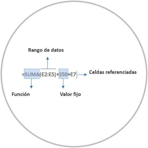
2 How to do a sum in Excel
To do a sum in Excel, we have seen some examples of how to perform this operation and in various ways. Before performing an addition operation, we must think about whether it is a simple operation between cells that are not contiguous, that is, that they are not one after the other. In this case we would use a simple formula to be able to add the corresponding cells, as in the example that you can see in the image:
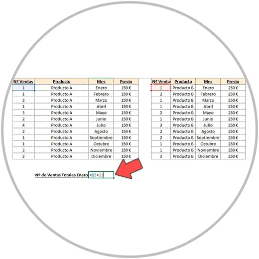
In the example, two specific cells are added in order to obtain a specific result, which is the number of total sales for the month of January for Product A and Product B. Continuing
with the example, if we wanted to make a sum of all the sales of a product, throughout the year, we could use the sum function because they are data that are collected in the same column. By carrying out an order and organization of data in columns, we can easily use a function, in this case of addition, to obtain the expected results..
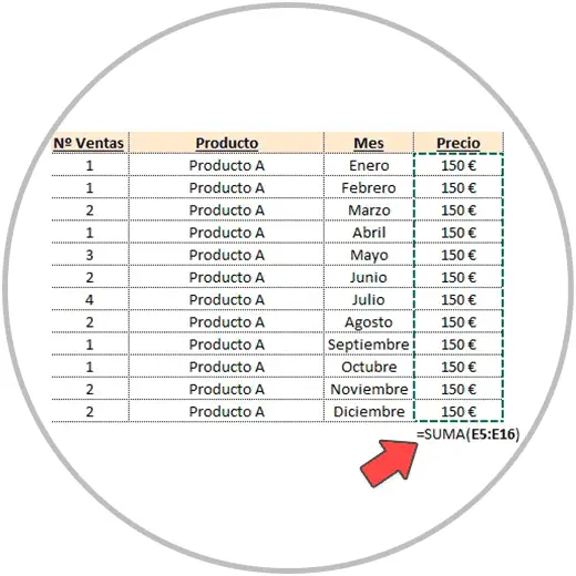
autosum function
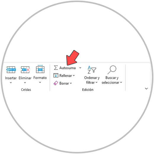
To do this summation, you can use Excel's autocomplete function, or we can go to the ribbon in the "Formulas" menu to find the desired function. Or we can also use the “Autosum” function, an option that we will see in the Start menu, on the ribbon.
3 How to do a subtraction in Excel
In order to do a subtraction in Excel, we are going to use the easy way to make a formula in Excel. There is no specific subtraction function in Excel, so, in order to perform a subtraction operation, we are simply going to follow the same procedure to perform a simple addition, using in this case the ”-“ sign, which we can see on our keyboard. . We can subtract fixed numbers, or we can subtract cells using, as we already know, the mouse or the mouse to select which cells we want to include in the operation.
If we wanted to subtract a range of data, remember that, as we already explained in how Excel works, we would have to first convert the numbers into negative numbers, and then use the addition function that we have already explained.
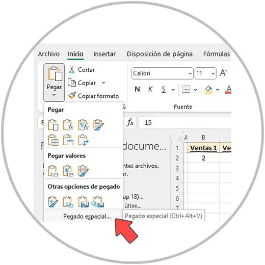
If we want to use the addition function to perform a subtraction, we will convert the values to negative. To carry out this process, remember that we have to copy the cell or cells to convert, using the keyboard to press the Ctrl + C keys. Immediately afterwards, we go to another cell where we want to paste the values, and from the ribbon we enter the “Start” menu and look for “Paste”. In the "Paste" menu, we look for "Special Paste"..
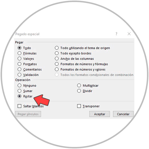
Now in the special paste window, we locate and mark "Subtract", as in the image and click "OK". Now we will see in the chosen cell how the negative values have been pasted.
4 How to do a multiplication in Excel
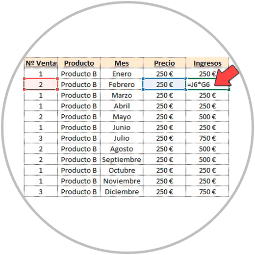
To be able to do a multiplication in Excel, we will follow the same process, introducing the “=” sign first, as we always do to start a formula; Then we will write the number that we want to multiply, or the cell where the value to be multiplied is, followed by the “*” sign; And then we would choose the cell where the other value to be multiplied is, or the fixed value to be entered in the formula.
Important
Remember that it is preferable as much as possible to always use references in the formulas instead of introducing fixed values. Usually, the tables, reports that we make in Excel become a file that we update frequently. To avoid errors, miscalculated data, it is preferable that whenever we use a formula, we use values referenced to cells.
Since we already know what the syntax of a formula in Excel is like, and how to use the operators or signs of operations in the formulas, we will be able to perform any other mathematical operation, such as division.
How to make a division in Excel
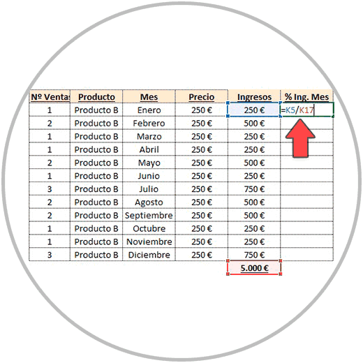
In order to carry out a division in Excel, we will use the same "modus operandi" as, in a multiplication, choosing if possible the cells that we are going to include in the operation, instead of including fixed values, separating the values or references to cells with the “/” sign, as you can see in the image:
Once an operation has been carried out in Excel, when we press the "Enter" key on our keyboard to see the result of the formula, we can assign the format that corresponds to that cell where we have made the formula. In many cases, the format that we are going to see by default is not the correct or the most appropriate. When interpreting the data and presenting a job well done, we must apply to each cell and column the type of format that best represents the information it is displaying. To change the cell format, as we already know, we have mainly three ways:
- Clicking on the cell where we want to change the format, with the right button of our mouse. We will then see a quick menu at the top of the window, from where we can change the cell format, and from where we can also configure the "look & feel" of the cell by choosing a background color, or establishing a format for the lines of the cell.
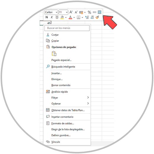
- From this window that opens when we click the right button of our mouse, we will also see the “Format cells” option in the menu.
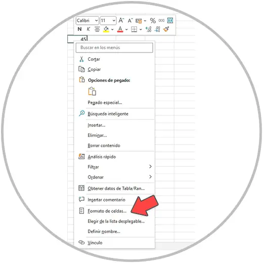
- From "Cell format", you can assign any format to the cell
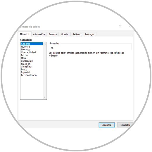
How to change the format of multiple cells in Excel
Remember that we can make the change in a single cell, or that we can select a range of cells to apply a common format to all of them. In order to change the format to several cells in Excel, we will select with the mouse or the mouse the range of cells where we want to establish a certain format, and we will follow the same process. We can also use the right mouse button to display the options for changing the format, or we can go to the start menu on the Excel ribbon, and choose from the drop-down the type of format that we want to apply to our cells or range of cells .
In this way, we can apply any format to our cells or ranges of cells.
5 How to get percentage in Excel
In order to get a percentage in Excel, we are going to carry out the same exercise that we have just carried out. Getting a percentage in Excel is a task that we can carry out by changing the cell format: using the right mouse button to access the quick cell format menu, or to enter the "Cell format" options. , as we have just explained.
We could also use the ribbon, and specifically the start menu to be able to use the drop-down window that allows us to choose a certain format, or we could use the visible option that we are going to see in the format section, within the start menu , like in the image:
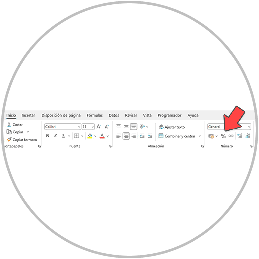
In any case, and as we have said before, we have to think about the format that best suits the type of information that we are showing in the column or in a specific cell. When we apply a percentage format in Excel, we must have the same mentality and check the data that we are going to convert into a percentage.
When we work on a data table, it is common, for example, to use percentages when calculating ratios. When we have values that are not currencies, or that are values less than 1, let's think about whether that column or row would be better represented by applying a percentage format.
When we perform a formula in Excel, we will get the result of the operation performed, or we may encounter an error if we have done something wrong, we are missing some element in the formula, or if we are trying to perform an operation that is not possible.
6 Fix formula errors in Excel
Next, we are going to see common errors that we can find when making a formula. These are very common errors that we are going to encounter when we make a mistake at some point when performing a formula or function or when we are trying to perform an operation that is impossible to carry out.
- #N/A: A typical error when we are performing a search operation and Excel does not find a value.
- #WORTH! It is surely the most repeated error in Excel, and it happens when we are doing an operation that cannot be performed, when for example in a mathematical operation such as multiplication we are using text instead of numbers. If we multiply, for example, the value of a cell by another cell that contains text, Excel will show us this error. To change it we will have to modify the formula or the cells referenced to others that contain numbers and not text. We can also find this error when we use an operator or sign in an operation that is not valid, or when we are making a formula and one of the referenced cells contains an error.
- #REF! This is another of the most common errors in Excel that usually occurs when we delete a cell, column, or row that is part of a cell. To solve it we will have to either delete the referenced cells that no longer exist from the cell or undo changes to return to a state before deleting the cell, column or row.
- #NAME? This is also a typical error that we will commonly see when we make a mistake when typing the name of a function. Here the autocomplete function is very important because if we get used to using it, it is an error that we can avoid, since we cannot make a mistake in the name of a function when we double click on one of the suggestions that Excel shows us.
- #DIV/O! When an impossible operation such as dividing a value by 0 is performed, we will see this error, which we will have to fix by modifying the value of cell 0 or by changing the cell referenced in the formula. It is also very common to encounter this error when, for example, we are performing a division and we are using a referenced cell that is an empty cell.
- ####### When we see hash marks in a cell, it's probably not an error. It is displayed when the value obtained as a result of the operation is too large to be displayed in a cell.
In any case, to solve the errors in these formulas, we can always move to the cell that contains the error, and place the cursor over the warning icon that Excel shows us, as in the image.
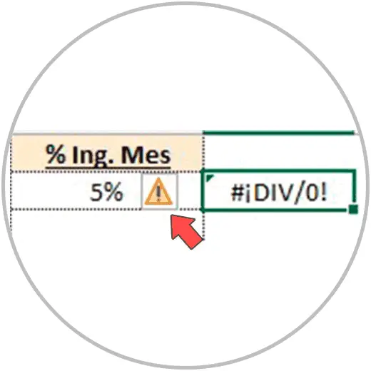
In this way it will tell us the problem. If we click on the warning icon we can get more information and help about the specific problem we have encountered.
Important
Remember that, in order to review a formula, we can move to the cell that contains the formula to review, and double-click on the cell; Or one that we place ourselves on the cell where the formula to be reviewed is located, we can also press the “F2” key on our keyboard.
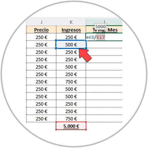
If we want to change a cell referenced in a formula, we will have to double click on the cell that contains the formula, or press the “F2” key. The cells referenced in the formula will then be highlighted, which, using the mouse, we can modify and change to another cell. We just have to drag the colored "highlight" of the cell from one of the edges, and drag it to the cell we want to reference, as in the image below. Or we can manually change the cell reference from the formula itself.
The use of formulas in Excel is a task that we will have to learn, just like in order to drive a car, we have to learn the theory, but also in practice, learn how to use the steering wheel, change gears and brake. The formulas in Excel are the resource that will allow us to better analyze the information, build the data table and report that we need, with all the ratios, KPIs, and values of interest that are necessary when judging the data objectively. .
On some occasions we will find that we have to build tables from scratch, and we have to add columns and rows to our table, performing some calculations to analyze the results; In other cases, we will find ready-made data tables that we will have to review, edit, correct, and that we will have to complete with new calculations.
Through the formulas, we can carry out calculations and simple mathematical operations, but we can also carry out some operation, which we will see later, with the help and use of the functions.