In Excel, the use of functions, as we already know, allows us to perform simple and complex calculations, and also allows us to save a lot of time and effort when performing tasks, especially when they are repetitive. By using functions, we can do mathematical operations such as addition, subtraction, average, we can obtain the maximum or minimum value of a range of data, we can perform the mean, median, and many other numerical operations in order to obtain valuable data. for analysis..
However, we already know that functions are also useful for performing other operations, such as performing conditional formulas that are very useful for evaluating results.
There are also other useful functions in Excel that are not used to perform mathematical or numerical operations, but that are very useful, and are frequently used to perform operations that would be impossible to perform if we had to do them by hand. This would be the case of the VLOOKUP (or VLOOK UP) function, a function frequently used by people who usually work on analysis tasks, and people who work with a large volume of data. VLOOKUP is a function that, whoever knows it, uses it frequently due to its great usefulness and the competitive advantage that comes with using this function..
The VLOOKUP function is very useful when searching for data, as it allows us to search for a concept and bring us information when we are working on joining or merging data, when we are trying to put together information that is found in different tables, on different sheets or in different files . They are useful when we want to build a single database, or when we want to build a data table by taking information from other sheets or files.
1 What is VLOOKUP in Excel
VLOOKUP or VLOOKUP is a tremendously valuable function when we work in Excel that is used to search for a specific value in a range of data, column or table and that returns a value that is within that range of data, in another column.
VLOOKUP is a function that goes beyond being a useful function to search for a value since by using this function we can bring valuable information. We can therefore say that it is a useful function to search for a value and extract information associated with that specific value..
Thus, we can build tables, or complete tables, searching for information found in other sheets or even different files.
What we can do with VLOOKUP
Next, we are going to see some examples of situations in which LOOKUP V would be very useful to achieve our goal:
- Cross data: When crossing information found in different tables, sheets or files, LOOKUP V is very useful. When we have related information, but it is separated into different tables. With VLOOKUP we could search for all the values of a column in another range of data from another table and bring us the information from another column.
- Search for information in a large volume of data: If we work with large volumes of data, finding a value can be a complicated task; Although there are ways to search for information using the keys on your keyboard (Ctrl + B), with VLOOKUP you can search for a value and get information or data related to that value you are looking for.
- Always updated information: Being a function, VLOOKUP allows you to have a table or report updated when performing this search and data extraction task is a task to be performed frequently and regularly. This way, you could, for example, maintain a list of updated products with prices that change frequently. For example.
These functions, in summary, allow us to have more resources when working with data tables when we want to complete the information in a table with information from another related table, when we have to make reports prior to the analysis, to be able to put it all together. the information in the same table, in the same report.
2 How to do a VLOOKUP in Excel
The VLOOKUP formula follows a language logic that you will be able to understand better with the image that we are going to show you.
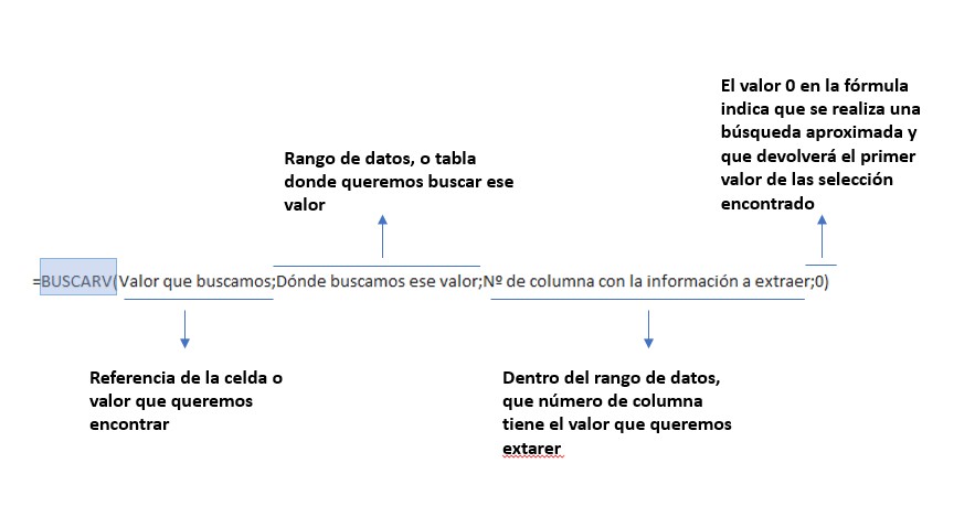
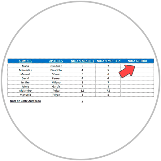
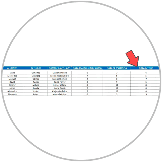
In order to use the VLOOKUP formula, follow these simple steps, following the same logic that we have shown you in the image. Next, in the example, we are going to see with images, how we carry out the VLOOKUP formula step by step to complete a table that has information about the grades of the students of a center. To complete this information, in the table where we have the information on the semester grades, we are going to build the VLOOKUP formula to bring us the attitude grades of each student that is on another sheet of the same file.
Steps to use VLOOKUP in Excel:
Let's see in the example what steps we must follow to build the VLOOKUP formula:
- As we already know, we start the formula by writing the “=” sign or the “+” sign in the first of the cells where we want to bring that information.
- Next, we start typing the name of the VLOOKUP function. With the Excel “autocomplete” utility, as we write, we will see the “VLOOKUP” function as a suggestion. We select it by double clicking on the name.
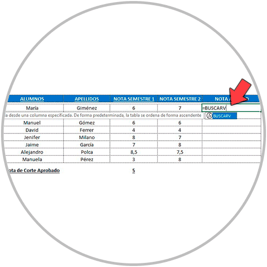
- By selecting “VLOOKUP” as a suggestion, we will see that it already places the name of the function in the formula and opens the parenthesis.
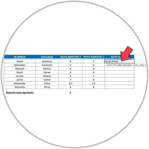
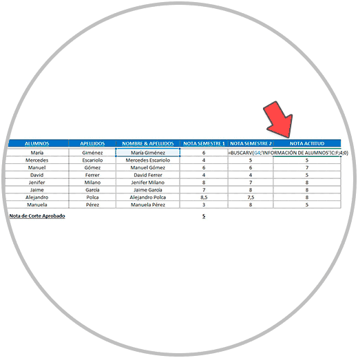
- Now is the time to write the value we want to look for in the formula. In this example case, we want to search for the student's name in another table, so, instead of writing, with the mouse we select the name "María" which is the first in the column containing the students' names.
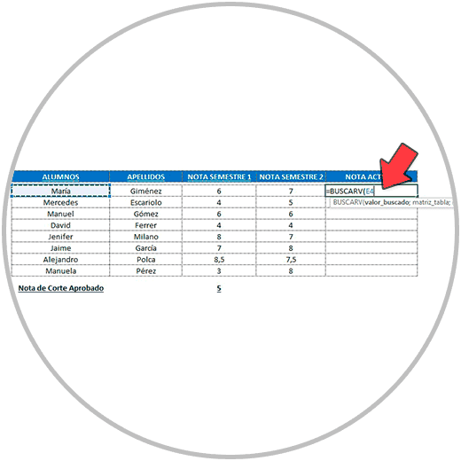
- Now we write the semicolon sign “;” to separate the value we want to look for from the next step, which will be to reflect in the formula “where” we want to look for that value. In this case, the value where we are going to look for the name of the students, to bring us the grade of their attitude, is on another sheet of the same file. We therefore open the document sheet that contains this information, and select all the range of data, taking into account that the first column of the selection must contain the names of the students. Look below in the image how we have selected the entire range of the table, from the first column that contains the names of the students.
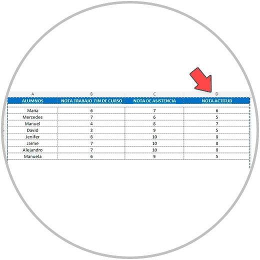
- Next, we write the separator sign “;” again and we put the column number that occupies the column where the information we want to bring is located, within the selected data range. Keep in mind that this point is very important, and we must write the number that it occupies within the selection or selected data range. In this case, as you can see below in the image, the “ATTITUDE NOTE” column occupies 4th place, and therefore in the formula we must put a “4”.

- Now we will complete the formula by putting the semicolon “;” back. first. Then, we will write a zero in the number “0” and close parentheses. As in the image below, this is what the formula looks like in total, after all the parameters have been included.

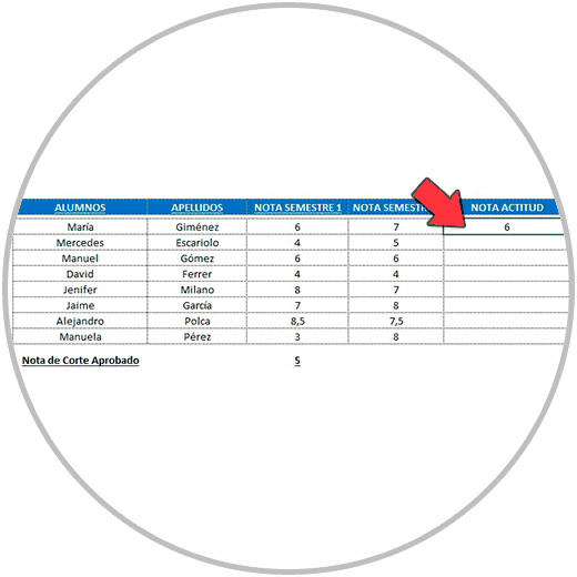
- Now when we press enter, we see that the formula works and brings us, in this example case, the behavior grade of the student “María” (which is a 6).
- Now, to get the score from the rest of the students, all we have to do is stretch the formula as we already know from the lower right corner of the cell.
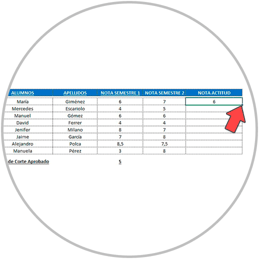
- And we stretch the formula by holding the click until the last row of the table we are working on:
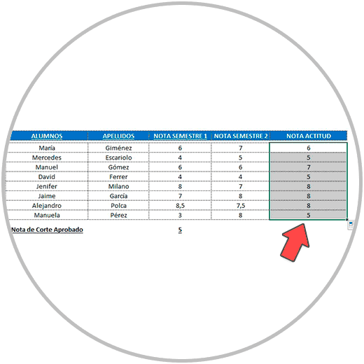
As we can see in the image, the formula has been stretched correctly, and in each row we now have the information with the attitude grade of each student that we have brought from another table.
How to use VLOOKUP in Excel from one sheet to another
When we want to use VLOOKUP to bring us a value that is in another sheet, we have already seen in the example how to do it. We have to carry out the formula naturally, following the steps, and when we get to the part of the formula where we have to select the data range, we will use the mouse to open the Excel sheet where the data we want to bring is. Just as we have done in the example.
Likewise, when the data is in another file, the procedure we will perform will be exactly the same. When we have to select the data range, we will use the mouse to open the document where the data is and be able to select the data range. Once the data range is selected, we must continue writing the next part of the formula.
3 How to do a VLOOKUP with two conditions
When we are making a formula with the VLOOKUP function, a situation may arise in which we need to take into account the information from other columns before performing the data crossing for the operation to be carried out successfully.
These are cases where in the same column, we have values that are repeated. When we want to search for values in other tables that are repeated.
This would be, for example, according to the exercise we just saw, if we had several students with the same name. In order to cross-check information correctly, we would have to take another condition or factor into account. In that case, we could, for example, take into account the surnames of each student, so that each value we are going to search for is a unique value.
The same thing happens to us in the column where those values are where we are going to search for those values. For the information crossing to be correct, we already know that, in the two tables, and following the example, when we talk about a person, and we want to cross the information, this name must be exactly the same on both sides. Now, what do we do then in those cases where, for example, we have several equal values in the same column? The solution would be to make these values unique, in the example using a cell that has the first name + last name information. If it happens that the surnames are in another column, what we would do is concatenate the column where the first and last names are. Let's look at the example below, how we would do it:
Steps to concatenate two cells in Excel
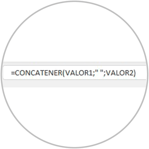
The syntax of a formula in which we are using the CONCATENATE function would be like this, like the one we show you in the image:
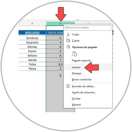
Let's apply this formula in the example we are seeing. We have added a column with information on the first last name of each student. (Remember when we add a new column in an Excel sheet, this new column is added to the left of the column we have selected.
We will then go to the letter of the column where we want to add the new column, by clicking with the right button. We will see that the entire column is selected, and a menu is displayed, where we will have to click on “Insert” if we want to add a new column.
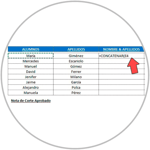
- We enter the “=” sign in a cell
- We start writing “CONCATENATE”.
- When we see that the autocomplete function gives us the name CONCATENATE, we select it by double clicking on the suggestion.
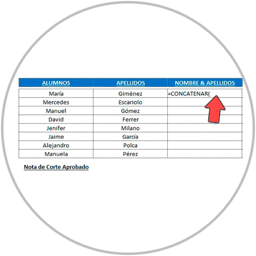
- We have to see that we have already opened parentheses in the formula, and now we must first put the value to concatenate, which would be the name of the student.
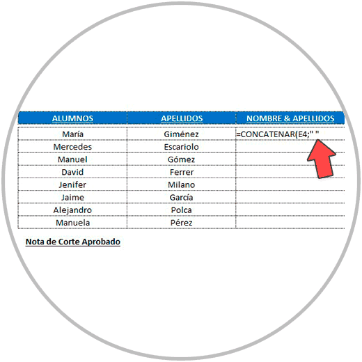
- Then, we include the separation sign that we use in the cells “;” and we are going to open quotes (“) add a space with the space bar, and we are going to put quotes again (“) Like in the image below. In this way we are adding a space in the concatenation.
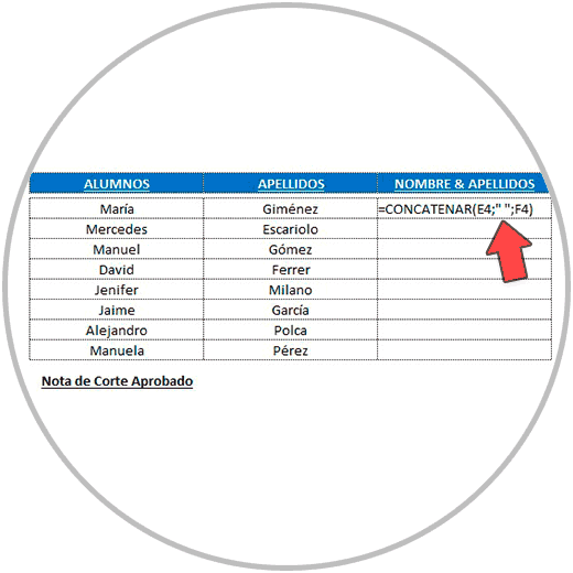
- Now we add another separation sign “;”, and select the other cell to concatenate, which is the last name, and we would close the formula with the closing parenthesis “)”, as you see below in the image.
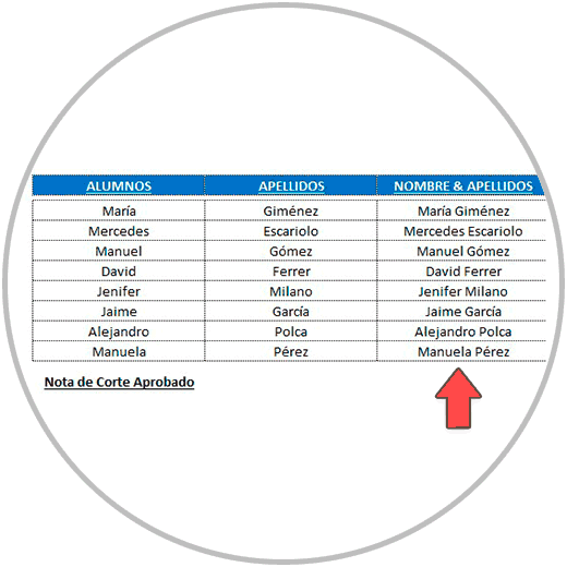
- Now by pressing the enter key on our keyboard, we will obtain the result of the formula. In this case, we will see the first and last name in a cell, separated with a space, thanks to the use of the concatenate function.
- Now we just have to stretch the formula downwards (remember that by clicking and holding from the lower right corner of the cell where we have made the formula) to be able to concatenate the first and last name of the rest of the students.
- Now that we have the first and last name concatenated in the Excel sheet where we are going to do the VLOOKUP formula, we would need to do the same (concatenate the first and last name of the students) in the Excel sheet where we are going to search and extract the grade. attitude.
- Now it no longer matters that there are students who have the same name. When performing the VLOOKUP formula, we would use this cell concatenated with the first name and last name, to search for the attitude note that is on the other sheet where we have already performed the concatenation of the first name with the last name.
- We therefore perform the formula again, this time first selecting, as you can see in the image below, the cell we want to search for, which will be our concatenated cell.
- We stretch the formula to the row that contains the last student on the list, and we check that the results are correct.
As you have seen, in this simple way we can take two conditions into account in a formula when we want to use VLOOKUP.
[/panelplain]
Both the VLOOKUP function and the CONCATENATE function are two of the most used functions in EXCEL due to the usefulness they have, even more so when we work with a large volume of data. In the examples, we can see how these functions are useful using them with simple data tables. Thus, the examples show how to use these functions more clearly. But let's think about how useful these functions would be if we were working with large data tables, continuing with the example, with larger lists of people, how useful these functions can be.
Let us remember that, in order to achieve the expected results, it is always recommended to use functions and formulas to perform operations and carry out tasks, whenever possible, to the detriment of more manual use. Imagine if we had to build endless lists of people, searching for their names in other files, and having to write down by hand the result we are looking for. How impractical it would be, and the mistakes we could make along the way, as well as the time we would need to carry out these operations.
For all these reasons, using formulas and functions whenever possible will help us work more professionally, faster, and better avoid typical errors.