As we all know, Microsoft Excel is integrated with a series of practical and dynamic functions with the objective of managing in a much more centralized way each aspect of the recorded data. One of these functions known to most of us is the VLOOKUP function which is integrated into the search functions of Excel 2019 and its mission is to find a value within a range of indicated cells. With this function, the search is done on values ​​located in a column so that it can also be called as a vertical search and hence the name of the function begins with the letter "V"..
The VLOOKUP function is ideal for finding items in a table or a range per row.
VLOOKUP arguments
The Excel 2019 VLOOKUP function has four arguments, three are mandatory and only one is optional. These arguments are:
- Lookup_value (Required): This parameter corresponds to the value we are looking for within the range we have selected and that will be compared with the values ​​in the first column of the table.
- Table_array (Required): Refers to the data table in which the search will occur. This table has both the values ​​to be compared and the values ​​that will be returned by the VLOOKUP function.
- Col_index_num (Required): Indicates the column number with the values ​​that are returned as a result of the search. The first column of the search range is assigned the number 1 and so on.
- Range_lookup (Optional): It is a logical value that proposes whether you want to do an exact search (FALSE) or an approximate search (TRUE).
Important items at VLOOKUP value
To consider when using the VLOOKUP function in Excel 2019:
- The searches using VLOOKUP from Excel 2019 are always executed from the first column of the range that we have selected taking into account that we cannot modify the variable. If where we are going to perform the search does not correspond to the first column, we will have to change the order of the data within each column so that the function is executed correctly.
- When the VLOOKUP function is executed, the result thrown will always correspond to the first match of the desired value. It must be taken into account that we cannot have several matches returned at the same time.
How to use the VLOOKUP function in Excel 2019
Step 1
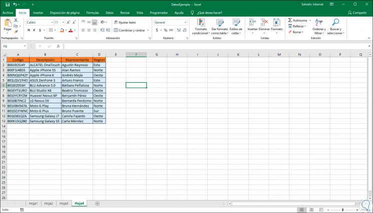
For this case we have the following information. There the range A1: D13 will be the general search range and column A, which is the first of this range, is where the search will be conducted according to our criteria.
Note
Something important to keep in mind is that the VLOOKUP function is the same VLOOKUP function in Excel 2019
Step 2
Now, we are going to perform a search where we throw the product according to the code entered, in this case we will execute the following. In this case, we have directly entered the value to search between Ҡand as we see the result is the product located in column 2.
= VLOOKUP ("B00J0O5J4Y"; A1: D13; 2; TRUE) Step 3
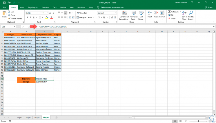
Another option we can do with VLOOKUP. It is to use a specific cell as a reference. In this way it is enough to enter the element to look for in that cell and not directly in the formula. In this case the term to be searched will be entered in cell C17 so that the formula will be as follows:
= VLOOKUP (C17; A1: D13; 2; TRUE)
Step 4
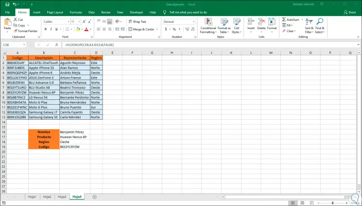
Remember that based on the result we want to obtain it will be necessary to specify the column. For example, if we want the representative's name to be displayed with the code entered, which is in column 3, the formula will be as follows:
= VLOOKUP (C17; A1: D13; 3; FALSE)

Step 5
We can also use different lines with their respective cell numbers to obtain the desired information:
Step 6
Some errors that we can find when using VLOOKUP are:
Common mistakes in VLOOKUP
- If the VLOOKUP function is instructed to return a column number that exceeds the maximum number of columns in the search range, the #REF! Error will be displayed.
- In case the value of the third argument of the function is zero, as if the function is indicated to return the column zero, we will get the error #VALUE!
- When performing an exact search, that is, when the fourth argument of the function is FALSE, but the function finds no match of the searched value, this will result in error # N / A.
- Error # N / A can also be displayed if the data type of the searched value and the first column of the search range do not match.
Thus, we have seen how the VLOOKUP function is useful and practical to perform an exact search for a term in a given range of rows and columns..