Microsoft Excel 2019 is part of the Office suite which has been developed by Microsoft with the aim of offering its millions of users the possibility to manage, manage and control data in a dynamic, comprehensive and with the best search results and of truthfulness. One of the tools most used by users is Excel. Without a doubt it is a very useful tool in terms of data management..
Excel has a number of functions, which allow you to perform different tasks quickly and easily. When managing large amounts of data , it is normal that you need to search for certain terms in a specific range or on the entire sheet (or pages of the book) to detect where that term is. For this reason Excel 2019 integrates two known functions that are VLOOKUP and VLOOKUP to execute the desired terms in a fully functional way.
TechnoWikis will explain in detail how we can make use of these two functions in Excel 2019 and thus have the best tools in terms of search terms..
1. How to use VLOOKUP function in Excel 2019
The VLOOKUP function (Search Vertically), is a function that is useful when it is necessary to find elements in a table or range per row of Excel 2019.
Step 1
Thanks to the VLOOKUP function of Excel 2019, it will be possible to find the desired value in a selected range either exactly or approximately, when using VLOOKUP we will be able to find a data in a table and thus determine if that data exists or not there in the search range that has been applied in the formula.
The syntax to use with the VLOOKUP function is as follows:
VLOOKUP (Search_value; search_array_array; column_indicator; order)
Step 2
These parameters are:
Wanted_value (mandatory)
There the data to be found in the selected range is indicated and this default value will be analyzed from the first column of the data range that we have defined, for a more concrete search Excel 2019 allows us to enter the text in quotes (Ҡ) or we can also use the cell reference where the value to be searched will be typed. Something to keep in mind is that the VLOOKUP function does not differentiate between upper and lower case letters.
Matrix_search_en (mandatory)
This parameter indicates the reference of the range of cells where the search for the desired term will be executed with VLOOKUP.
Column_ Indicator (mandatory)
In this parameter we refer to the column number from which the result will be obtained according to the assigned formula, so when the VLOOKUP function detects that there is a match of the data to be searched, it is responsible for returning the result that is entered in the column assigned in the VLOOKUP formula.
Order (is an optional parameter)
This parameter is a logical value, that is to say false or true, its function is to tell the VLOOKUP function the type of search to be executed, it can execute an exact search (FALSE) or an approximate search to the result (TRUE). The default value of this argument is TRUE.
Before using the VLOOKUP function it will be necessary to take into account some conditions that the data must meet, these are:
- First, the data to be managed must be organized vertically, that is, in column format, since the VLOOKUP function has been developed to analyze the data vertically until it detects the value that we have registered in the Excel formula 2019.
- The VLOOKUP function executes the search for the desired element from the first column of the selected data range and it is not possible to modify this behavior.
- If there are more data tables in the same Excel 2019 sheet where the search is to be carried out, we must leave a row and a blank column between the data where the search will be carried out so that the VLOOKUP function use only the range where the search is to be performed and do not take additional values ​​from other tables as it may result in an error.
Step 3
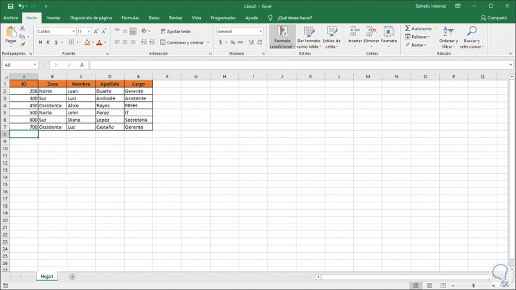
For this analysis we have the following data:
Step 4
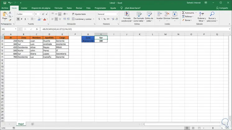
In this case we will detect the zone by entering the respective ID, for this, in cell H1 the zone will be displayed and in cell H2 we will enter the respective ID, for this case the syntax to be used will be the following:
= VLOOKUP (H2; A1: E7; 2; FALSE)
The syntax we have used has been the following:
VLOOKUP
Indicates the type of search, in this case vertical.
H2
Refers to search by the value entered in cell H2 in the indicated range
A1: E7
It is the reference to the range of cells where the search for the desired term will be executed.
two
This value indicates the column number from which the result of the selected range will be obtained.
FALSE
Indicates the accuracy of the search where True refers to an approximate search and False refers to an exact search as we have mentioned.
Step 5
For example, if we enter ID 300 in cell H2 the result will automatically be South in cell H1:
Step 6
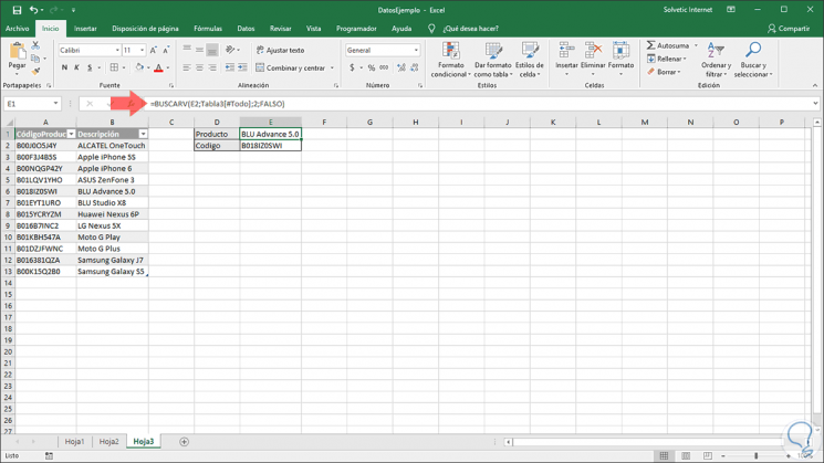
It will be possible to use the VLOOKUP function with any range of cells as long as we enter the correct data:
Common mistakes when using the VLOOKUP function in Excel 2019
There are some errors that we can receive when using this function, these are:
- In case the key column does not have the unique values ​​for each row, the VLOOKUP function will return the first result found that matches the searched value.
- If we enter a value equal to zero in the column indicator, the VLOOKUP function will return an error of type # VALUE!
- If a column indicator greater than the number of columns in the table is indicated, an error of type # REF!
- If the VLOOKUP function is configured in order to execute an exact search, and the desired value is not found, the function will return an error of type # N / A.
- Thus, we have learned to use the VLOOKUP function in Excel 2019.
2. How to use the BUSCARH function in Excel 2019
Unlike VLOOKUP, this VLOOKUP function is responsible for searching for a value in the top row of a table or an array of values ​​and returning a value in the same column of the row indicated in the table or matrix. SEARCH (Horizontal Search), will search for a value within a specified range, and if it fails to detect any value, this will result in a # N / A error.
Step 1
We can use this BUSCARH function when the value to be searched is in a row of the data table, if not, the VLOOKUP function performs the search in a specific column.
The syntax of this function is as follows:
SEARCHHR (value_search; array_search_in; row_indicator; [ordered])
Step 2
The indicated parameters are as follows:
Wanted_Value (Required)
This is the value to look for in the first row of the table. This parameter can indicate a value, a reference or a text string since all of these are compatible with BUSCARH.
Matrix_search_en (Required)
This parameter is the Excel 2019 table where the information to be found is found, this table or range will be analyzed by BUSCARH to launch the expected result, there we can make use of a reference to a range or the name of a range and the values ​​of the first row of the argument can be of type text, numerical or logical values.
To take into account the following, in case the ordered parameter is TRUE, the values ​​of the first row of the range where the search will be executed must be entered in ascending order, otherwise, SEARCH will return an incorrect value. If the ordered parameter has the FALSE command, it will not be necessary to sort array_search_in.
Rows_ Indicator (Required)
This parameter refers to the row number from which the value that matches the criteria recorded in the formula is to be obtained. If the indicator is 1, it will return the value of the first row, if the indicator is 2, it will return the value of the second row and so respectively, now, if the indicator of the rows is less than 1, SEARCHH will result in the error value # VALUE !; If the indicator is greater than the number of rows in the selected range, SEARCH will return the error value # REF !.
Ordered (Optional)
This is a logical value where we will indicate whether BUSCARH execute a search with exact or approximate match of the value to be searched. If this parameter is omitted, its default value is TRUE.
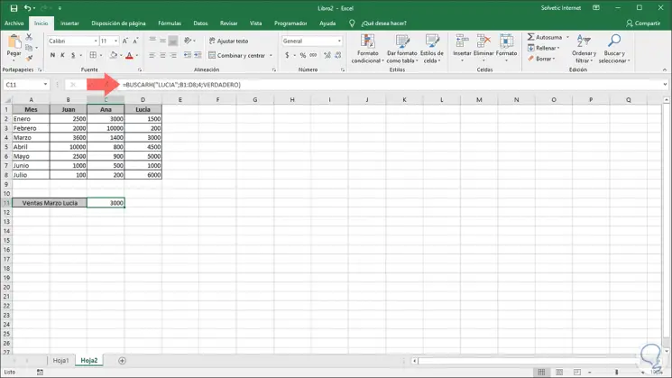
Now, for this example we have a series of monthly sales data of various employees, if we want to know Lucia's sales in March, we execute the following formula:
= LOOK FOR ("LUCIA"; B1: D8; 4; TRUE) There, the first argument is “Lucia†since it is the person we are looking for, with the second argument we enter the range of data without including the month column (column A) since it is not vital, in the third argument we refer to the row number in which you want the SEARCH function to generate the result, there we must enter the row number of the month or value to be searched and finally enter the desired search value based on the type of result to be obtained, the result will be the next:
Some tips to keep in mind with the BUSCARH function:
- If the SEARCH function does not find the searched and ordered_value is TRUE, it will use the highest value that is less than the searched_value.
- If the desired_value is less than the lower value of the first row of the_search_array, SEARCHH will give the error value # N / A.
- If the order is FALSE and the value_search is a text value, it will be possible to use the wildcard characters of question mark (?) And asterisk (*) in the argument value_search, there the question mark refers to a single Any character and the asterisk is equivalent to any sequence of characters.
As we have seen, the functions BUSCARV and BUSCARH in Excel 2019, are really practical for the whole specific process of terms and thus achieve the best results. It is a way to access all this information quickly. No doubt Excel is always a good option when we are referring to data management.