Question

How to calculate the subtotal, VAT and Total in Excel 2019 and Excel 2016

Answer 1

How to calculate the subtotal and VAT in Microsoft Excel 2016 or Excel 2019

---

Microsoft Excel , either in its 2016 or 2019 editions, is used for a wide range of tasks, from the creation of dynamic tables to the control of large databases. All this in a safe and truthful way thanks to the various functions and formulas integrated within the application..

Thanks to its practicality when making calculations , Excel becomes the best alternative for the management of some obligations that we must generate or fulfill and one of these is neither more nor less than the VAT which is a tax that the government establishes about a high percentage of products and services so that each of them is legal.

On many occasions when we must apply VAT to a product, we do not know for sure how to perform this task. For this reason, TechnoWikis will explain through this tutorial how to calculate not only the VAT of a product but also the subtotals taking as criteria the data supplied..

We leave you as a complement the video to be able to calculate a price that has VAT from Excel 2019 or Excel 2016.

To stay up to date, remember to subscribe to our YouTube channel! SUBSCRIBE

How to calculate the subtotal and VAT in Microsoft Excel 2016 or Excel 2019

This tutorial will be done in Excel 2019 but the same steps must be applied if we use the 2016 version..

For this we have the following data where we have created a column for the subtotal, the VAT and the global total which is the sum of both the subtotal plus the VAT:

Calculate the subtotal of products

The first step we will take is to calculate the subtotal of the products, which is simple. To do this we must multiply the quantity by the value of each product, place our cursor in cell D2 (Subtotal column) and execute the following formula:

 = B2 * C2 

As a result we will see the subtotal of the selected product:

We can drag the formula to the lower cells so that it is copied and the operation is executed:

Calculate the VAT of products

Up to this point we have defined the subtotal of the products and it is time for us to calculate the VAT which is 21%, for this, we go to cell E2 and we have the following options to execute the VAT calculation:

• Subtotal * 21/100
• Subtotal * 0.21
• Subtotal * 21%

For this case we will use the Subtotal * 21/100 syntax with which we will enter the following in cell E2:

 = D2 * 21/100 

As a result we will see the value of the VAT of this product:

Like the previous method, we can drag the formula so that the value is automatically applied to all the other cells in the selected range:

Calculate the cost of products

With subtotal and VAT defined, it is time to determine how much is the total cost of the product which is determined by adding the columns Subtotal + VAT, in this case we enter the following in cell F2:

 = D2 + E2 

We can drag the formula again to automate the process in the following cells:

Calculate the VAT of products with multiply

In addition to the steps suggested by TechnoWikis the VAT may be calculated in other ways which we will explain in detail so that your knowledge is complete.

One of these options is to enter the VAT in a cell with the format 21% and then multiply the price by said VAT, for example, we have entered 21% in cell B8, so that in cell E2 we execute the following:

 = D2 * B8 

There we can copy the formula for the following cells but we must keep in mind that if we use this method. Cell B8 will continue to increase, which in cell # 3 we will see the formula = D3 * B9 and as a result will be an empty field since there is no VAT assigned, in this case we must use the absolute function and it is useful when our list is broad, that is, it contains many fields to apply the VAT, there the use of the absolute value of Excel is ideal since it will fix the selected cell.
If we did not use it, we would see the following:

To avoid this and perform the function with the VAT of cell B8 without it being altered, we will enter in cell E2 the following syntax:

 = D2 * $ B $ 8 

To achieve this we can enter the $ signs manually or place the cursor in the middle of B8 and press the F4 key:

After this if we can copy the cell and the B8 value will remain static:

Automatically add VAT

An essential point that has Excel 2016 or 2019 is the diversity of functions, another method to automatically add the VAT of our product is to automatically add these values. This is possible because the percentages are basically a decimal value and 100% refers to the number 1, so we are going to multiply the subtotal that we have already made by 1 plus the percentage of VAT in cell B8 like this:

 = D2 * (1 + B8) 

As a result, we will see that with this method the VAT has automatically been added to the global subtotal:

From then on we can copy the formula to the other values.

Know the cost of a product before VAT

A point that many of us may find somewhat complex is knowing the cost of a product before VAT. For this Excel comes to our aid and determine the value of a product before VAT we must execute the following, defining that in cell B8 is 21% VAT:

 = E2 / (1 + $ B $ 8) 

As a result we can see that the generated value is equal to the one registered in the subtotal of the products:

Format and sort data with table

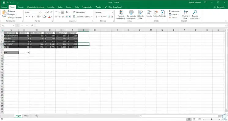
As we can see, the options to calculate the VAT are varied. Now, if we want to apply a much more professional format to the registered data, it is possible to apply a table style to the rank to be able to exercise certain attributes there.

To achieve this, we will select the range of data and use the following keys and the following pop-up window will be displayed where it will be possible to validate the data range:

+ T Ctrl + T

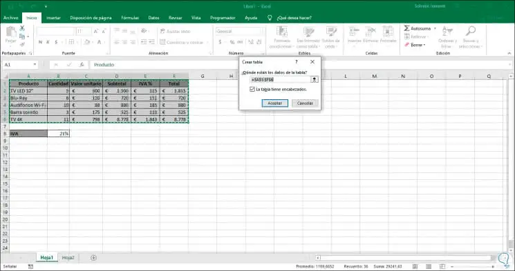
Click on OK and we will see that this format is applied and we have a new menu called "Table Tools" where we can edit the style of the table, the data, etc:

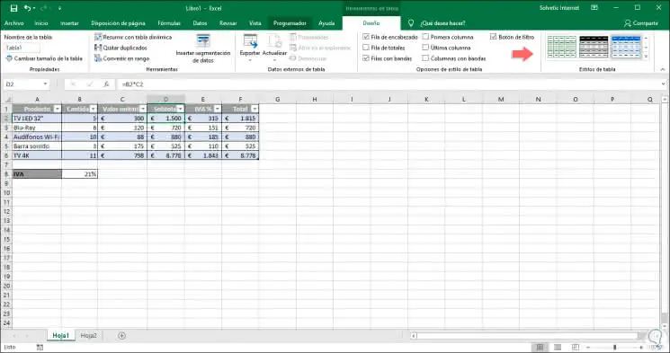
One of the great advantages of this format is that we have filters which can help us to explicitly visualize a product and its details:

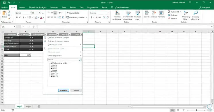
Also with the filters it will be possible to order the data as necessary, from least to greatest or vice versa:

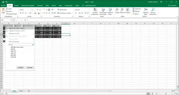
Thus, if we choose from lower to higher we will see the changes automatically:

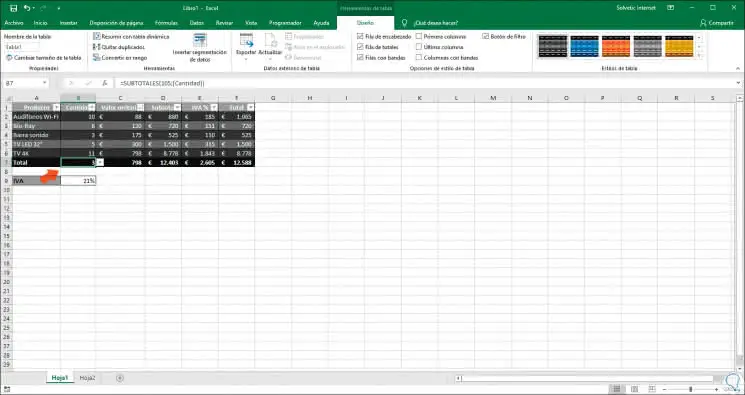
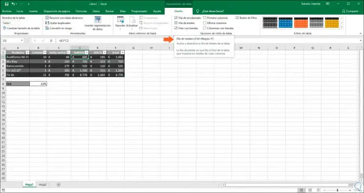
Another point to keep in mind with the table is that we can automatically insert a row of totals to see the sum of the values ​​in our range. To do this we click on the table and go to the menu "Design-2 and in the group" Table style options "find the box" Row of totals ":

Note

We can use the following keys for activation:

+ O + T Ctrl + O + T

By selecting this box, we will see how the "Total row" is inserted with the sum of the "Total column":

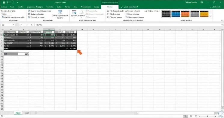
To add the other values, we will click on the respective cell and in the drop-down menu we select "Sum":

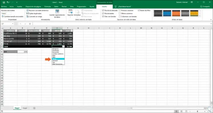
For this example, we have selected "Sum" in the columns "Subtotal and VAT" as well as the Minimum value in the column "Quantity and Maximum" in the column "Unit value":

We see how Microsoft Excel gives us the necessary tools for precise and accurate calculations of both VAT and subtotals.

---