Microsoft Excel is one of the most dynamic and complete applications for the execution of hundreds of tasks associated with numerical data . Undoubtedly one of the applications that users use most is Excel. Thanks to this data manager, the possibilities of performing different operations are immense and very useful. More than 80% of the data entered and registered in Excel are of this type, where each one plays an important role and from which we can perform multiple operations based on the requested requirements..
Many users go to Excel to create tables from which to record different data, add and subtract dates , create drop-down lists , make a pivot table or create a calendar . No doubt the options offered are immense.
Microsoft Excel, both in its 2016 and 2019 versions, provides us with a set of functions to calculate addition, subtraction, higher values and one of the practices, especially in the financial field, is to calculate averages and for this Excel provides us with multiple options for that end..
TechnoWikis will explain through this tutorial how to calculate and obtain averages in Microsoft Excel in a simple and functional way.
Note
This process applies equally to Excel 2016 as 2019.
1. How to calculate averages using the Excel 2019 or Excel 2016 table format
Step 1
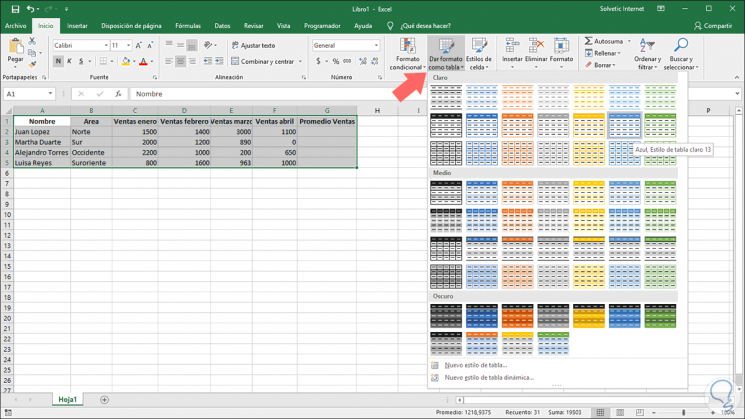
The first option involves converting the recorded data to the table format and from there performing the process. For this method, we will select the data to calculate and go to the Start menu and in the "Styles" group we click on the "Format as table" option and in the options displayed we select the most appropriate for our report:
Step 2
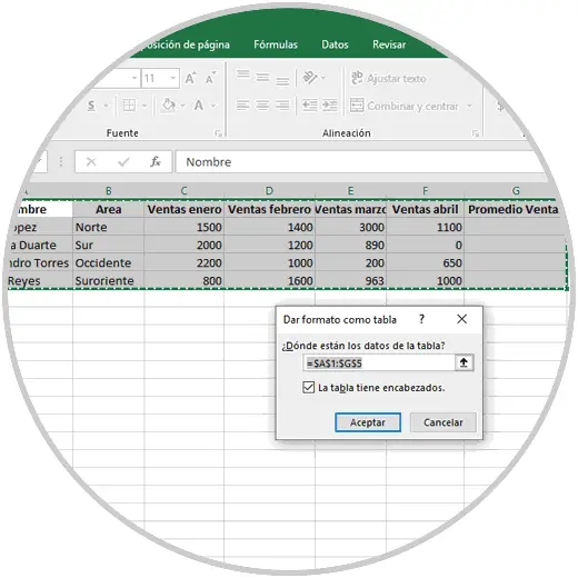
When selecting the style, a pop-up window will be displayed where we can view the selected data and if necessary edit it:
Step 3
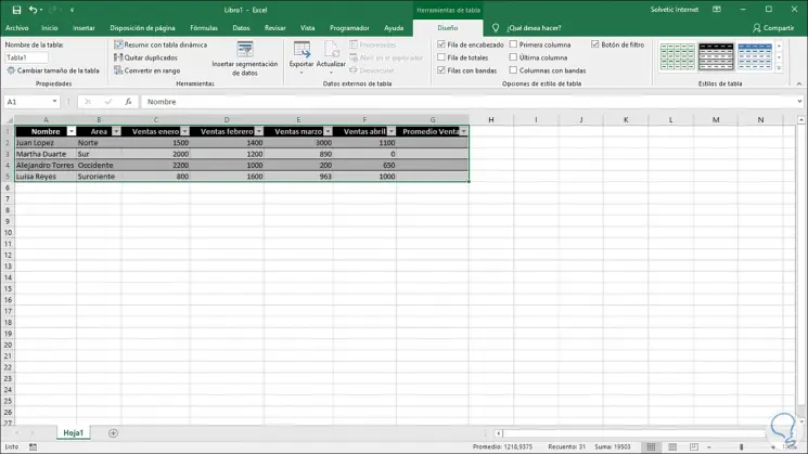
Click on "Accept" and the table format will be applied to the selected data:
Step 4
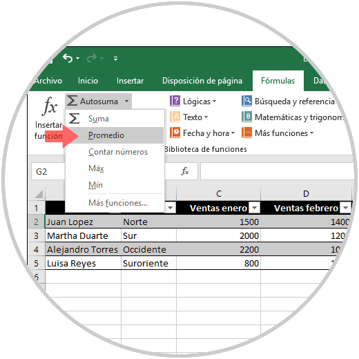
Now we place the cursor in the first cell of the "Average Sales" column (in this case), and we go to the Formulas menu and there, in the "Function Library" group, click on "Autosuma" to select the Average option :
Step 5
When you do this automatically Excel will detect the numerical values ​​in the table:
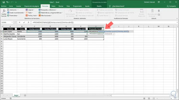
Step 6
Press "Enter" to confirm the action and this formula will automatically apply to the entire table:
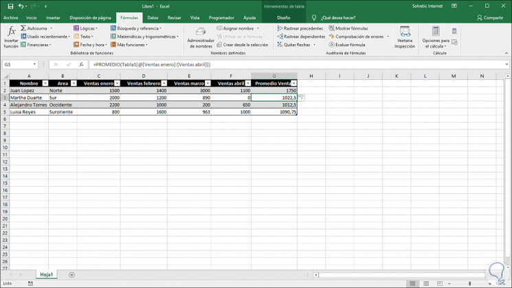
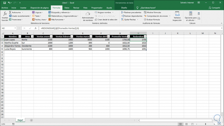
As we can see, these values ​​are calculated based on the recorded data. We are likely to want to round these out in order not to have decimal values ​​in the result. If this is the goal, we can go to a new cell and use the round function..
Step 7
For this we place the cursor in the desired cell and in the Formulas menu we click on "Function Library" and there we click on the "Mathematics and trigonometric" category and in the displayed list we look for the Rounded function:
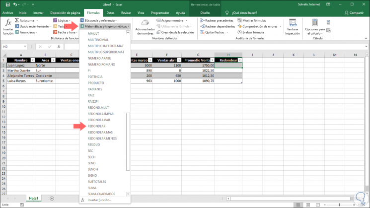
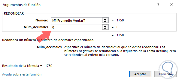
Step 8
When selecting this function the following wizard will be displayed where we must enter the arguments of the function, there we register the following:
- In the Number field we click on the Average Sales column
- In the field Num_decimal we enter the value zero (0)
Step 9
Click on "Accept" and this function will automatically be applied to all cells in the table:
2. How to use the Average function in Excel 2019 and Excel 2016
Microsoft Excel 2016 and 2019 integrate a function called average which is a function that has been developed to measure the central tendency, which is in turn the central location of a group of numbers in a distribution based on statistics.
There are three (3) measures in the scope of the trend which are:
Average
This value is the arithmetic mean which is calculated through the sum of a group of numbers and dividing by the totality of these numbers, for example, the average of 10.20 and 3, whose sum is 33, if this is divided by 3 the average will be 11.
Median
It is the average number of a group of numbers where half of the numbers have values ​​higher than the general average and half of the numbers have lower values ​​this same average
Mode
Refers to the most frequent number in a selected group of numbers.
With the Average function it will be possible to perform certain actions which we will see next.
3. How to calculate the average number of a row or adjacent column in Excel 2019 or 2016
Step 1
For this process we must click on a cell below or to the right of the numbers on which the average will be calculated, once the cell is selected, we will go to the Start menu and in the Edit group we click on the Autosuma option and there we select The Average option:
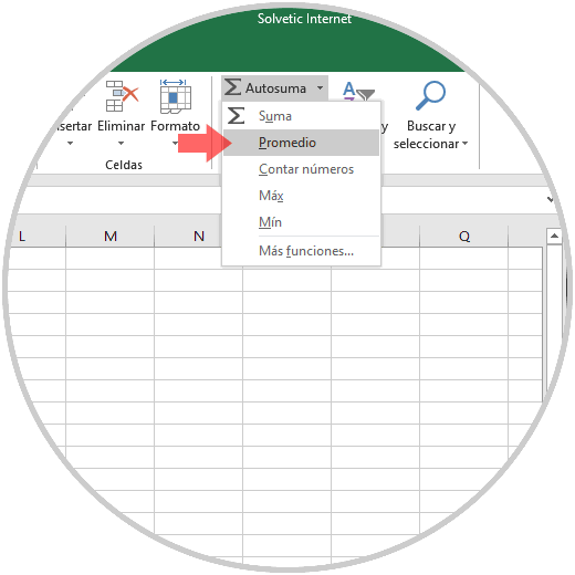
Step 2
Automatically Microsoft Excel will take care of the average of the numbers registered in the sheet:
Step 3
Press Enter and the average of this range will be displayed:
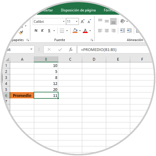
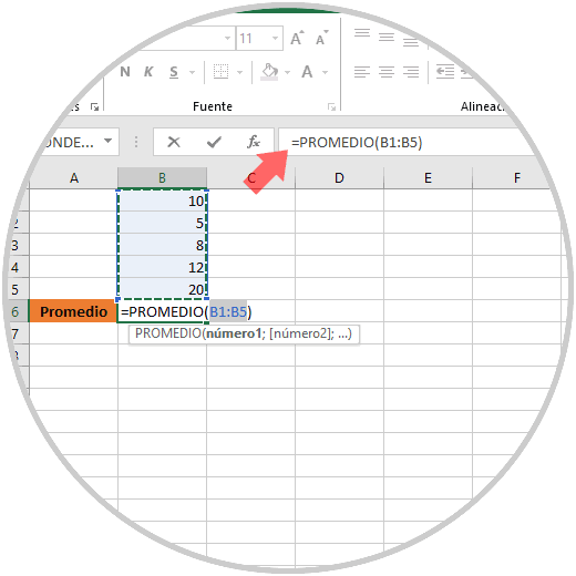
4. How to calculate the average numbers of a non-contiguous row or column in Excel 2019 or 2016
Step 1
It is likely that the data is in cells located in different cells within the spreadsheet, however, it is possible to make use of the Average function to obtain this result comprehensively.
In the previous case we use the following formula:
= AVERAGE (B1: B5)
Step 2
This formula finds the average of all the numbers in the indicated range, in case of having values ​​in different formulas we will execute the following formula:
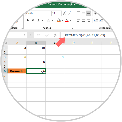
= AVERAGE (A1; A3; B1; B4; C3)
Step 3
In this case we have numerical data in the indicated cells, for this we enter = AVERAGE and use the Ctrl key to click on each of the cells that contain the data to be validated.
Step 4
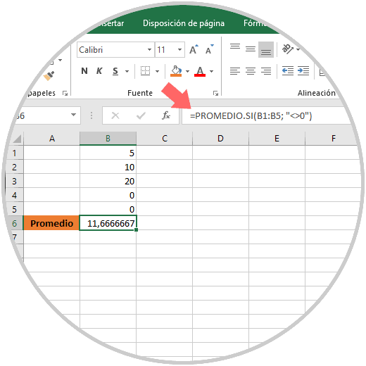
Another alternative is to use the following formula in this case:
= AVERAGE.SI (B1: B5; "<> 0")
This is responsible for returning the average of the indicated range except the cells that contain zero:
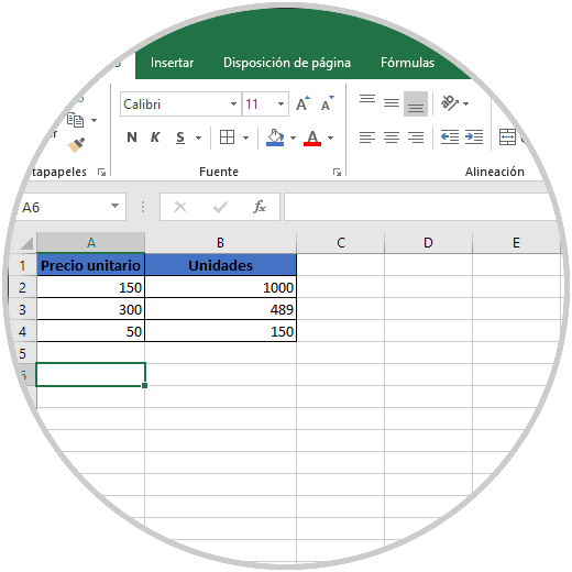
5. How to calculate the weighted average in Excel 2019 or 2016
Step 1
To calculate this type of average, we must use the SUMPRODUCT and sum functions and for this we have the following data:
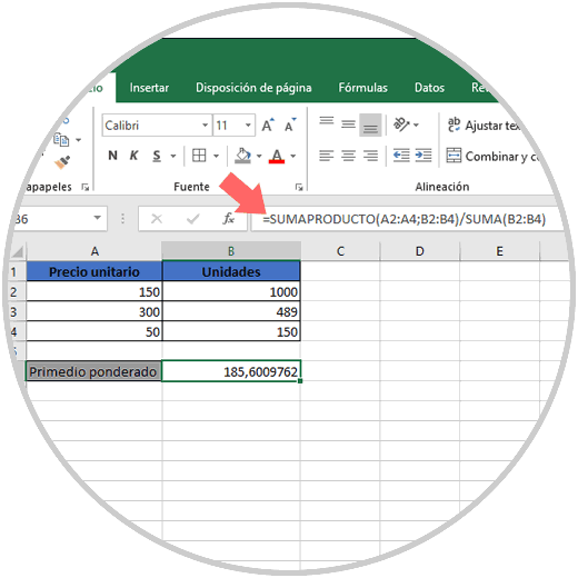
Step 2
There we will execute the following formula based on the recorded data: = SUMPRODUCT (A2: A4; B2: B4) / SUM (B2: B4)
This formula is responsible for dividing the total cost of the three elements by the total number of units assigned:
As we can see, the options to calculate the average in Microsoft Excel 2016 or 2019 are wide and their results are complete and true. In this way we will be performing a task that can take us a long time, simply and quickly.