Question

How to calculate percentage% annual growth rate Excel 2019

Answer 1

1. How to calculate percentage of the growth rate in Excel 2019 using the TIR.NO.PER function
2. How to calculate percentage of annual average growth rates in Excel 2019
3. How to calculate percentage of compound annual growth rates in Excel 2019

---

There are two words that in many users cause the same impact as a horror movie and these are "Excel" and "calculation of percentages". Now, it is even more terrifying if we say that we must calculate a percentage in Microsoft Excel 2019, the new edition of this office suite. But one of the functions that not everyone knows is that thanks to the functions integrated in Microsoft Excel 2019 it has the ability to calculate percentages, in this case calculate growth percentages. This function will be a simple task for the various tools that Excel 2019 brings with it and our horror movie will now be an action movie..

The percentage of the growth rate gives us the opportunity to analyze in detail the exponential growth using the existing data and in this way to determine if our project is viable or not, so we can make the best decisions regarding this.

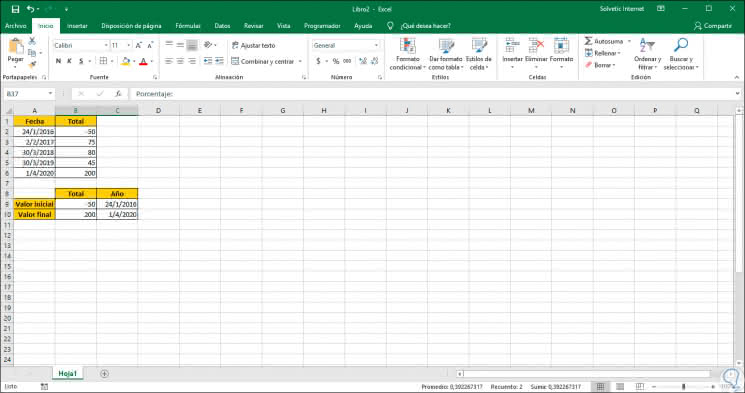
For this tutorial we have the following scenario:

Note

In cell B2 we have entered the value -50 since this is the initial investment of the project, it is mandatory that the first value is negative so that the execution and calculation of the formula is appropriate.

TechnoWikis will explain the available ways to achieve an integral and adequate calculation according to the real need for analysis. You also have the videotutorial that shows you the necessary steps to calculate the annual growth rate in Excel 2019..

To stay up to date, remember to subscribe to our YouTube channel! SUBSCRIBE

1. How to calculate percentage of the growth rate in Excel 2019 using the TIR.NO.PER function

This function TIR.NO.PER or XIRR (if we use Excel 2019 in English), is a function that has been developed with the objective of returning the internal rate of return for a range of data without it being mandatory that these are periodic.

Step 1

Its usage syntax is the following:

 TIR.NO.PER (values, dates, [estimate]) 

Step 2

The parameters are the following:

Values

It is a mandatory data and represents the range of data or cash flows which is actually a payment schedule that is linked in turn by the date parameter, it is ideal to understand that the growth percentage applies for cash values.

Within this parameter you must include a positive value and a negative value as minimums, that is, when we speak of a positive value we refer to is the investment and any cost or payment is understood as a negative value.

Dates

It is another mandatory value and this parameter refers to a schedule of dates which is related to the payments of the values, these dates can be defined in any order.

Estimate

This is an optional value within the function and is as such a number that we enter which is approximated by the result of the TIR.NO.PER function.

Confused? Do not worry that TechnoWikis will try to explain it so that you understand each point of the function.

Step 3

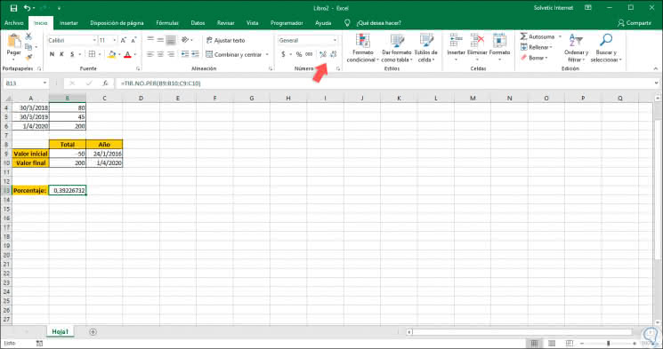
Based on the data in our spreadsheet, we will execute the following:

 = TIR.NO.PER (B9: B10; C9: C10) 

Step 4

There we will use the initial values ​​as well as the range of initial and final dates. As a result we will obtain the following:

Step 5

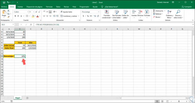
For this value to be converted into a percentage format we will go to the "Start" menu and in the "Number" group we click on the% icon and we will configure the number of decimals to use through the "Increase or Decrease" decimals":

Step 6

Some aspects to take into account with the TIR.NO.PER function:

• In case one of the numbers of the parameter dates does not apply as a valid date, the function TIR.NO.PER will return the error value # VALUE !.

• We must enter a negative value and a positive one, if not, we will see the error # ¡NUM !.

• In case the parameters values ​​and dates have a different number of values, TIR.NO.PER will result in the error # ¡NUM !.

Thus, thanks to this function we will be able to calculate our growth percentages in a dynamic way.

2. How to calculate percentage of annual average growth rates in Excel 2019

Step 1

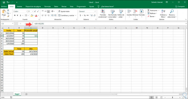
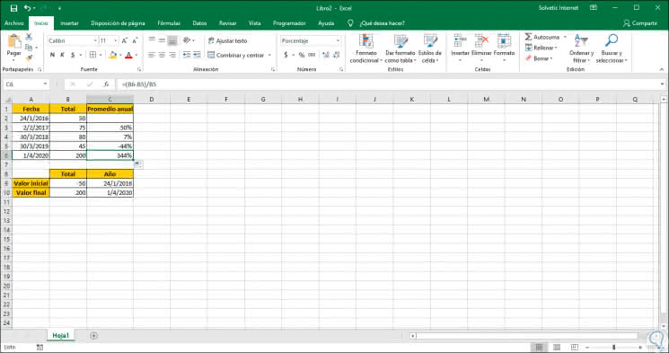
This is another method to calculate the percentage of growth since it is done annually, that is, each year, we can calculate the rates of each year registered by taking the criteria "Final Value - Initial Value / Initial Value", in our example we will use the following formula:

 = (B3-B2) / B2 

Note

For this case, negative values ​​are not required.

Step 2

Once we execute the formula we can go to the group "Number" to apply the percentage format and in step we can drag this formula to the following cells so that the growth of each registered year is analyzed:

Step 3

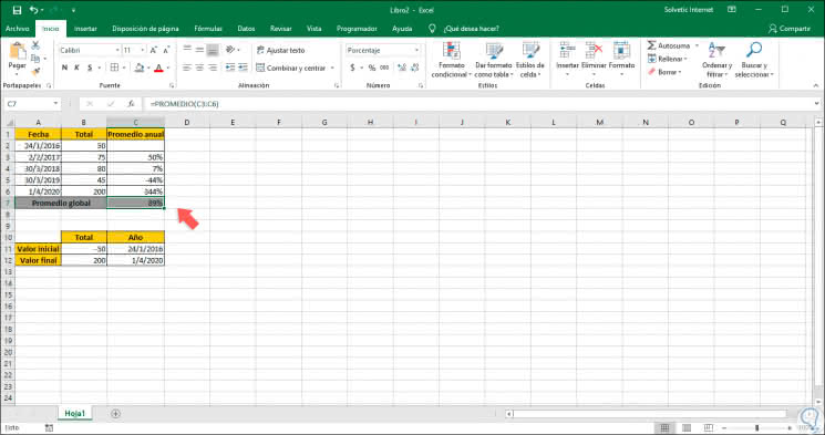
For more complete information we can add the general average with the following formula:

 = AVERAGE (C3: C6) 

3. How to calculate percentage of compound annual growth rates in Excel 2019

Step 1

This calculation is a function that is responsible for measuring the rate of return of an investment, based on an investment period of 5 to 10 years, to correctly use this function in Microsoft Excel 2019 we will use the following syntax:

 = ((Final value / Initial value) ^ (1 / (Periods - 1)) -1 

Step 2

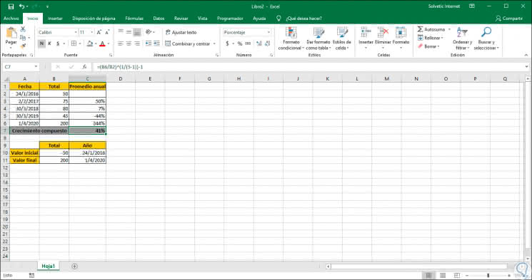
For our example we will use the following formula:

 = (B6 / B2) ^ (1 / (5-1)) - 1 

Step 3

Then we can apply the percentage format for a much more complete representation:

As we have seen, Excel 2019 and the calculation of growth is not something of terror that must torment us, thanks to TechnoWikis you will dominate it completely with the best results..

---

Answer 2

Growth rate simply explained
Calculate growth rate
How to calculate average annual growth rate
CAGR
Formula growth rate
Germany GDP growth rate
People's Republic of China GDP growth rate

---

How to calculate average annual growth rate

Growth rate

Here we explain in an easy-to-understand way what the growth rate is and how you can calculate the growth rate and the growth factor using simple  formulas .

Growth rate simply explained

By definition, a growth rate describes the relative increase in size over a period of time. It looks at the change in the current period related to the value of the previous period. If several periods are to be considered, an average relative increase in size per period, i.e. the average growth rate, can also be determined.

CAGR

The CARG ( C ompound A nnual G rowth R ate) is a special form . Translated into German, this means something like “compound,   annual growth rate ”. As the name suggests, this is the average percentage change per year. It plays an important role above all in business and economics when considering market development, sales and investments.

Calculate growth rate

The calculation of the growth rate is generally very simple. To measure the increase or decrease in size over a certain period of time, you need two numbers: a start and an end value.
You take the difference between the two values ​​and set them in relation to the starting value. So the difference is divided by the starting value to get the relative change .
There is also the growth factor. It describes the factor by which
the previous value (start value) must be multiplied in order to achieve the later value (end value).

Formula growth rate

If you summarize the above explained in a mathematical formula , it looks like this:

or

is defined here as the relative change in a value compared to its predecessor .

You can calculate the aforementioned average or   average growth rate over several periods as follows:

or

It thus represents the geometric mean  . If the variable is years, we speak of the CARG as already mentioned .

To get the growth factor of both formulas, omit that at the end of the formula:

Growth factor:

medium growth factor:

or

Germany GDP growth rate

In the following example, you calculate Germany's GDP growth rate and that of the People's Republic of China using the CARG. Then you determine the growth factor and compare the growth of gross domestic products .

You look at a period of ten years  from 2007 to 2017:

Germany GDP 2007: $ 3.440 trillion

Germany GDP 2017: $ 3.667 trillion

For the calculation you use the average growth rate. Since it is  years, however, it is called CARG. Put the values ​​in the first formula.

Germany's GDP has therefore grown by less than one percent annually within a period of 10 years.

To calculate the growth factor, you can simply add the CARG to 1:

The result can easily be checked by calculating backwards:

People's Republic of China GDP growth rate

For comparison, the same is calculated for the People's Republic of China.

People's Republic of China GDP 2007: $ 3.552 trillion

People's Republic of China GDP 2017: $ 12.240 trillion

The CARG is also calculated here, but this time you use the second formula:

The GDP of the People's Republic of China has grown significantly over the 10 years, averaging around 13% annually.

The growth factor is therefore 1.1317. This can also be checked again:

---