On a daily basis, the organization and management of different data is fundamental, both in our daily lives and in the workplace, and there are many programs that help us manage this information quickly and tactically. Among all of them, if one stands out for its ease of use, versatility of use and the large number of functions that allows us to perform is undoubtedly the program of the Office Suite , Microsoft Excel..
Many of us use Microsoft Excel , both in its editions 2016 and 2019, to manage large volumes of data in a practical way thanks to its various integrated functions. It is for this reason that it is a mandatory App on our computers (although many are terrified to hear the name Excel) for a reliable and effective administration of texts , dates , numbers and other elements.
Since the data to work is really high, and often complex, Microsoft integrated a function thanks to which the view of the details will be much more complete and simple and is the possibility of dividing our spreadsheet into panels. This will undoubtedly help all users who want an adequate management of each data since when dividing a sheet, it will be possible to move down in the lower panel and still not lose sight of the upper rows. This is something that happens when we have a data in row 205 but the goal is in row 2. This is the purpose of the division of leaves in Excel and therefore TechnoWikis will explain how to do it without losing your head and this process applies for same in the 2016 and 2019 versions of Microsoft Excel..
By default, Excel integrates the Divide functionality so that we do not become entangled in the work of the data. The best of all this is that by using this function Divide we will have full control according to the current visibility and work needs.
To stay up to date, remember to subscribe to our YouTube channel! SUBSCRIBE
Step 1
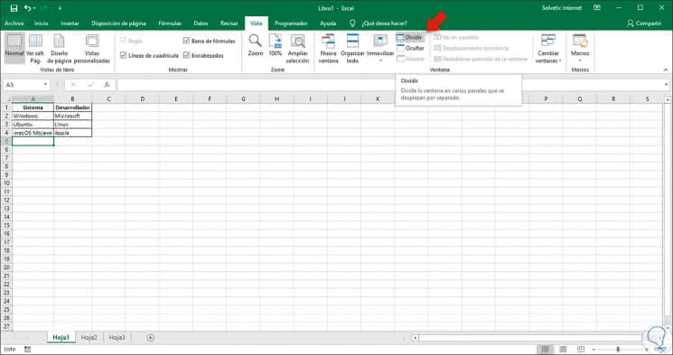
To make use of this option, we will go to the View menu and in the group "Window" we will find the option Divide:
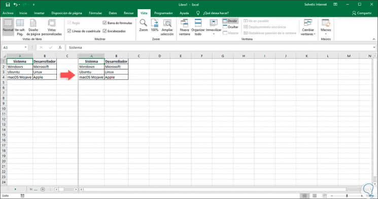
Step 2
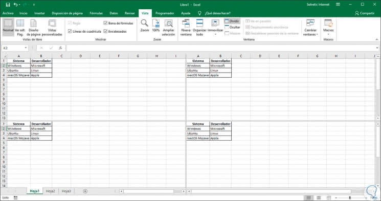
When clicking on it, we will see a series of lines since Microsoft Excel is responsible for dividing the active sheet into four quadrants with the same dimensions. What we will see will be the following. As we can see, there will be created areas of work where we can enter data to be used, but it is important to highlight that the original text will be copied in the four work areas, remember that before clicking on "Divide" we must select cell A1.
Step 3
These dimensions can be modified by clicking on the dividing lines and moving them as we deem necessary:
Step 4
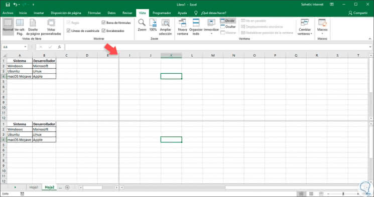
Now, we can also create the division horizontally, for that we select a cell different from cell A1 and the dividing line will start from there:
Step 5
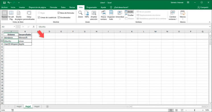
In the same way we can select a column and click on "Divide" and said segmentation will start from there:
Note
The original data will always be copied.
We must keep in mind that from where the cursor is located from there the spreadsheet will be divided in Microsoft Excel. When we consider that it is no longer necessary to use the Divide function in Excel 2016 or 2019 anymore, simply go back to the Window group and click on Divide..