To start using the Excel options, functions, formulas, as well as other applications and functionalities present in the Microsoft spreadsheet, we will need to open a new Excel document or we will have to open a document that we have saved on the computer, in OneDrive , on an external device or in a network folder..
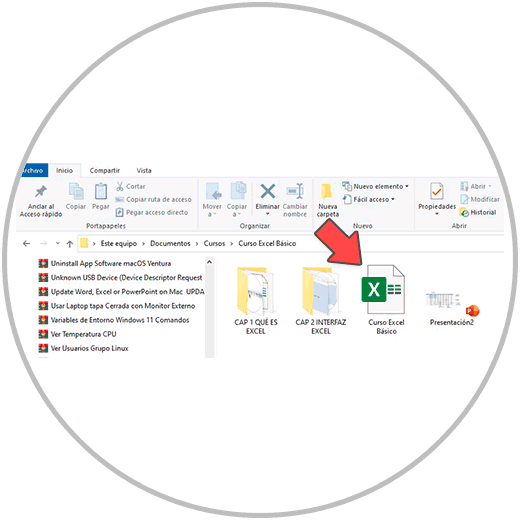
Whether we are going to work on a file that has already been created, or if we are going to start creating our file from scratch, the first thing we can do is open Microsoft Excel. If we are going to work on an already created document, we will open the folder where the document is saved, and we will double click on the document.
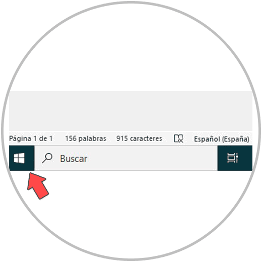
In case you want to start using Excel from scratch by opening a blank document, the first thing we are going to do is open the program from the beginning. To open Excel, we move with the mouse to the Windows button, located in the lower left corner..
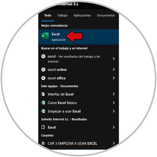
By clicking on the Windows button, we are going to search for the Excel application using the sidebar to Scroll until we find the Excel icon, as we can see in the image below:

How to Open Excel
To open Excel, we can also use the Windows search, using the window that is located just to the right of the Windows start button (in the lower left corner).
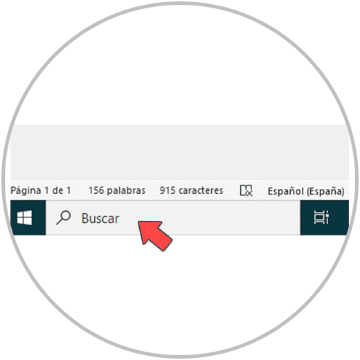
By clicking on the search window, we can write the word Excel to quickly locate the program, which we would open by clicking, as in the image, on the program icon.
Once Excel is open, we can start using its functions, tools and options to carry out our work..
As we already explained in what the Excel Interface is like, we can use the mouse of our computer, or the keyboard, to be able to scroll through the Excel menu. If we remember, in the upper bar (quick access toolbar) we have some options that we can configure; In the quick access toolbar, we have the Excel search box that we can use to find any Excel option, function or tool.
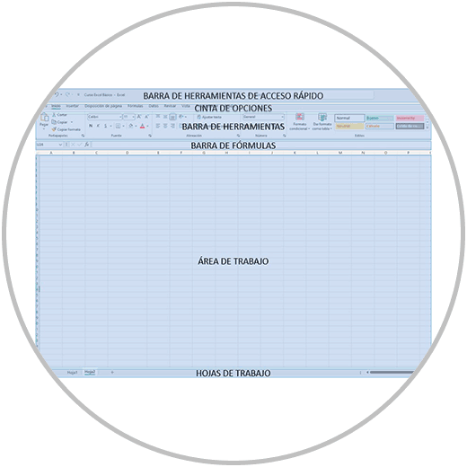
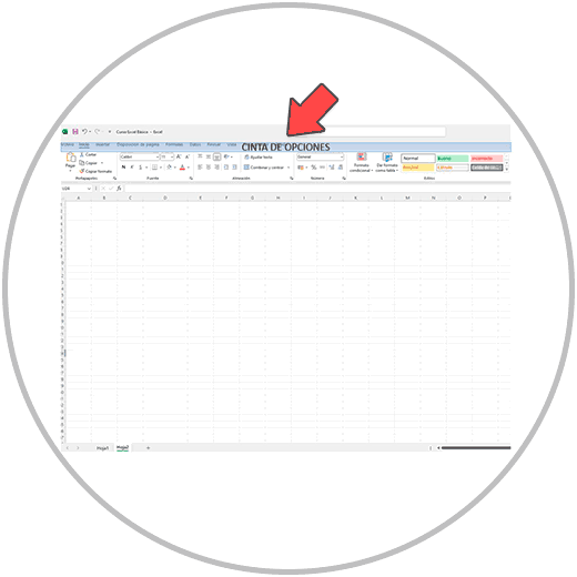
Also, from the ribbon, we will see all the options, tools and functions to use to configure our data, to shape it, create formulas, assign a format, etc.
1 How to start creating a table in Excel
Once we have Excel open, and we are clear about how we can move through the menu to be able to locate all the Excel options, we can start using the Excel work area.
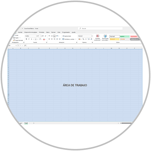
In the Excel work area, we will see that this part of the Interface is made up of cells. The cells in Excel are the rectangular spaces that we will see when opening any document. In the cells, as we are going to see below, we can write any type of content: we can write words or phrases (text), we can enter numbers, and we can also enter functions or calculate data using formulas.
In the cells, we can also include references to other cells, for example, to bring us a value from another cell of the sheet where we are working, or from any other sheet, whether or not it is in the file where we are working; But we can also use a reference to be able to include it in a formula and calculate a value.
The cells, as we already explained, are distinguished based on some coordinates or references using the location of the cell depending on the column and row in which it is located. If we look at the workspace, the column names are determined in alphabetical order, and the rows follow the same logic, but using numbers. Thus each cell will have a unique identity, which will be formed with the letter of the column in which it is located, together with the row number to which it belongs.
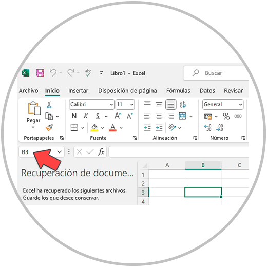
Thus, as we can see in the example image below, the cell that we indicate with the arrow would be cell "B3", because it is located in column B, and in row 3.
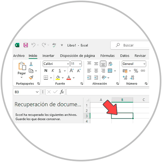
The cell coordinate, if we look closely, will be indicated to the left of the formula bar, in a window, as you can see in the image below.
The coordinates or references in Excel are very important because we are going to use them frequently in the formulas, in such a way that we can perform an operation using any cell in the document.
When we start using the work area, to write text, to enter a number, or to perform an operation in Excel, we are going to use the mouse or mouse and the keyboard of our computer. In this sense, as we already explained, it is not necessary to have to calculate the reference of a cell, but we will use the mouse or the keyboard to be able to indicate which cell we want to use.
2 Start writing numbers and letters in Excel
In order to start writing in Excel or entering numbers, we can place ourselves in any cell of the Excel sheet using the keyboard. By clicking on any cell, we can start writing using the keyboard; We can also use the numeric keyboard, to be able to enter numbers.
Recommendation
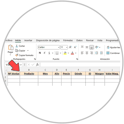
If you are going to build a data table, remember that the order and structure is very important, even more so if we are starting to build an Excel from scratch that we are going to use frequently. In order to keep an order, as we already explained what Excel is, we are going to build tables with a logic in which we are going to create some column headers that are going to indicate the type of information that we are going to add. Therefore, we work at the column level, establishing the headers with the names of the columns, as we have indicated, depending on the type of information that we are going to add to Excel.
Thus, for example, as you can see in the image below, we begin to introduce the headers of a data table that will contain information on the sales of a company, where we also find sales attributes such as the type of product sold, the price , where the sale took place.
How to move from one cell to another in Excel
To be able to move from one cell to another, you only have to use the mouse of your computer.
When we finish writing in addition to a cell, we can use the “Enter” or “Enter” key on our keyboard. By pressing the “Enter” key, we will move to the cell that is immediately below (we will move vertically).
In order to move horizontally, we can use the “Tab” key on the keyboard, which is the key on the left, represented by an arrow pointing up.
To be able to move from one cell to another, in summary, we can use, as you already know, several ways or methods:
- the mouse or mouse
- The Enter key, to scroll vertically down
- The “Tab” key or tabulator on the keyboard, to move horizontally in the right direction
- We can also use the arrow keys on the keyboard to move in the direction we want.
Important:
If when trying to move with the arrow keys on our keyboard, we see that pressing any arrow key prevents us from moving between cells, it is likely that we have the lock key active. We will solve it by pressing the Scroll Lock key
Scroll Lock
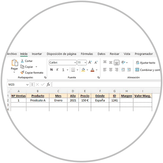
Continuing with the example, as we already know, we are writing in the cells and composing our table, entering text and number as appropriate.
3 How to make a formula in Excel
A formula in Excel is a code that we are going to create inside a cell to be able to calculate a ratio, or obtain a value or a result. A formula in Excel is an operation that is generally performed to obtain a result that will be important in order to analyze the results.
All formulas must begin with the equal sign “=” or with the plus sign “+”. Either one is valid. Yes or yes, formulas must start with the “=” sign or the “+” sign. This is how we are telling EXCEL that we are going to create a formula, and therefore Excel will be able to assist us, as we will see with the auto-completion functions.
The formulas must follow a syntax in which we manually enter the values, or we choose the cells that we want to include in the formula using the mouse or the keyboard.
What is the syntax of a formula in Excel?
We are going to use an example to be able to see all the elements that we can find and use within a formula. As you can see in the image, we found before a formula in which several elements that compose it can be distinguished.
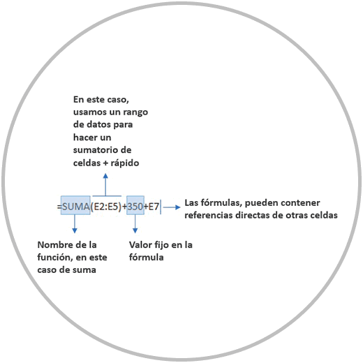
In this example, we find all these elements:
- Name of a function: in the example, we use the “sum” function; But we can use a multitude of functions to calculate ratios, perform operations, or obtain a certain value according to the need to obtain a specific result. There are many functions in Excel that are useful. Below we will explain how to find other useful functions.
- Data range: In the example, we also see a data range which is very useful in the formula to avoid having to add cell by cell. The combination of a function, plus a data range is perfect to save time, and make shorter formulas that are easy to handle. In order to include the range of data in this case, we use parentheses () and in between we are going to put from which cell to which cell we will perform the summation. This chaos is the perfect example of why we should always be very organized and try to build tables with very specific criteria in which we always work at the column and row level as we have shown you in the example. To be able to choose a range of data, the mouse will be very practical to be able to select a range,
- We also find a fixed value in the formula , because as we have said we can also do operations by entering a number “by hand”. When entering fixed values, we must take into account that, if this is a value that can change, we are not interested in using a fixed value, as it will remain in the formula and cannot be changed automatically. We will have to change it by hand.
In these cases, it is better to use “referenced values” in the formulas, that is, values that are found in other cells. Instead of putting fixed values, we introduce as in the example a reference to another cell so that it uses its value. In this way, the formula will always be updated if the value of the cell that we are referencing changes.
Finally, in the formula we find “signs of operations”. The signs of operations are those that mark, together with the functions, what type of calculation we want to perform. In the example we use the + sign of addition, but we can do multiplications, divisions, percentages %, etc.
4 Use Excel functions
When creating new calculations for our Excel tables, there are many functions that allow us to obtain a specific result. As an example, we have already seen how the sum function works, and how it saves us time when performing a calculation. We have also seen how it is interesting from a practical and productive point of view, since we do not have to select cell by cell, but rather we can select a range of data avoiding making mistakes, and also avoiding creating endless formulas when the summation requires the sum of many cells.
There are many functions in Excel, and there is a way to access all the functions that will help us choose the function that best suits the operation we want to perform thanks to "Insert function".
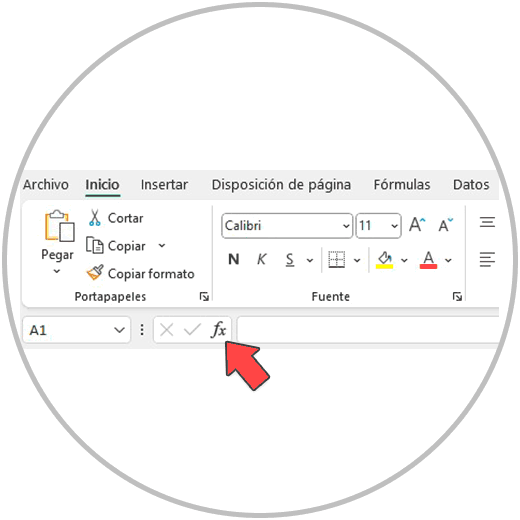
“Insert Function” is an Excel tool and assistant to be able to enter a formula. We can access this wizard with a single click because, as we see in the image below, it is always available to the left of the formula bar:
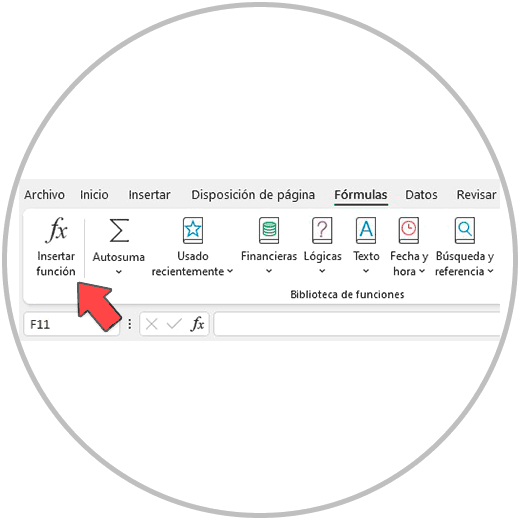
We can also open the insert function tool from the Excel ribbon, by clicking on “Formulas”. We will see on the left the Insert function symbol, on the left of the taskbar, as in the image:
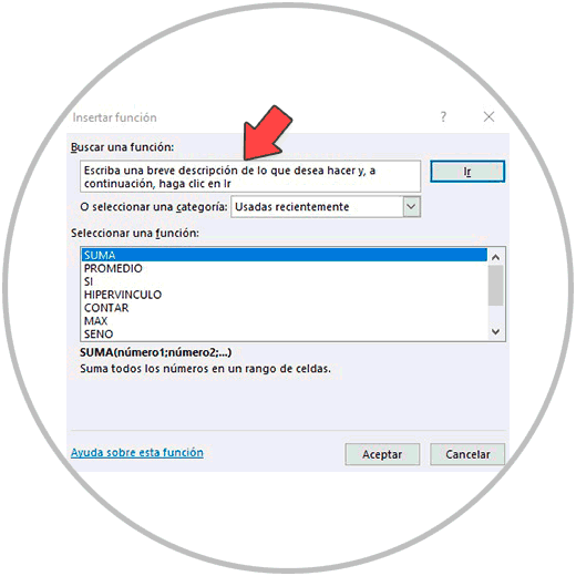
When opening the insert function tool, we will find a window from which we can write the name of the function or make a brief statement about the operation to be performed.
This function is very interesting to find a function, but let's not forget that when we are creating a formula in Excel, the autocomplete function will work in a similar way and will allow us to select it directly while creating the formula. In order to use the autocomplete function to select a formula, we must know the name of the function, or write the name of the operation to perform: If we want to add, we will start writing "add".
Simple operations such as subtraction, or multiplication, do not have a specific function to use. The sum does have it since, in a table, it is interesting to be able to perform the sum of an entire column, or the sum of an entire row. If we wanted, for example, to do a subtraction operation using a function, we could use the "Sum" function and convert all the values we want to subtract to negative.
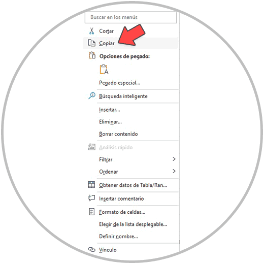
To convert a value to negative in Excel, we copy the value using the mouse and clicking the right button, choosing the copy option, or we are in the cell we want to copy and use the keyboard to press the Ctrl + c keys.
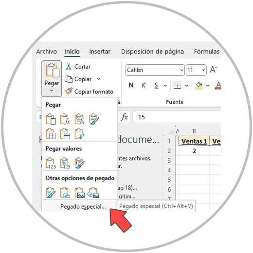
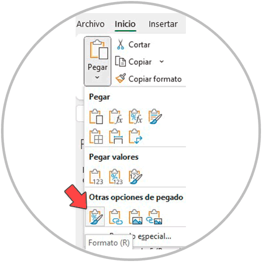
Now we would place ourselves in another cell, and we would go to the ribbon, clicking on “Start” and then on “Paste”. At the end, among the options, we will see "Special Paste" we would click on "special paste", as in the image:
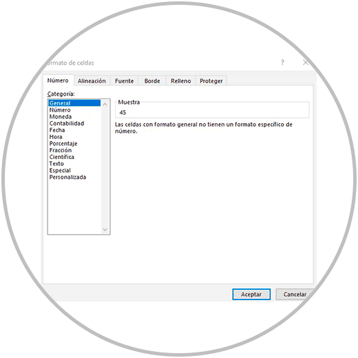
Now among the options, we have to choose the "Subtract" function, as in the image below, and click "OK". Now you will see in your work area, in the cell that you have chosen, how this value has been set in red and with the negative sign in front of it.
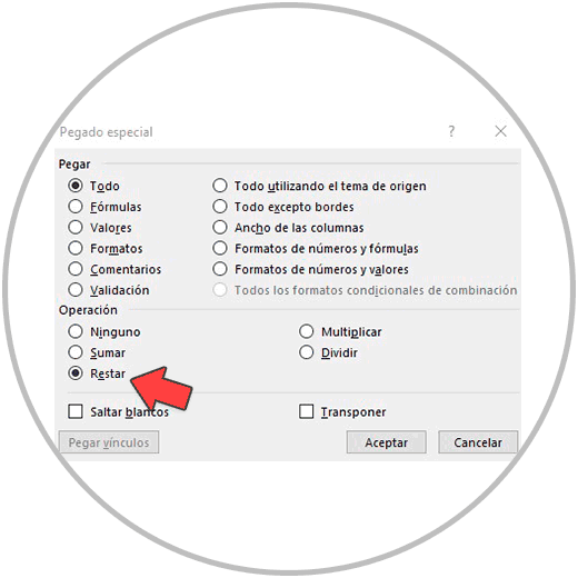
It is important that, once you have converted the value or values to negative, to perform the subtraction function you use the addition function. (or that you add the values cell by cell), but we cannot use the subtraction sign.
There are many functions that we will see in detail later, we will give you tips to be able to hit 100% with the formula and function to use, giving you some simple tricks that will make you infallible when creating any formula.
5 Format cells and tables in Excel
When we talk about formats in Excel, we can talk about the cell format. When we hear about cell formatting, we usually talk about the format of the cell's content. Depending on whether the cell has a numeric value or has text, we can apply different cell formats. Especially, when there are numeric values in the cells.
When we talk about numeric values, we are talking about the numbers that a cell can contain. These numbers, to see some examples, can be:
- Whole numbers without decimals
- Numbers in a given currency.
- percentages
- dates
To apply a cell format, we can mainly use 3 ways:
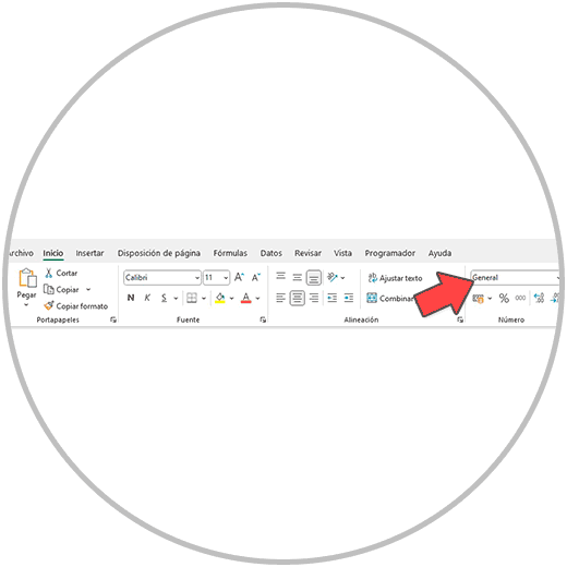
- Apply a format from the ribbon in "Home". As we see in the image below, using the options that we see inside Start in the drop-down window of formats.
- Also, we will use a very useful function, clicking on a cell or range of cells that we have selected. We will click with the right button of our mouse or mouse on the cell or range of cells where we want to apply a format. In the options that we see below when clicking with the right mouse button, we can use a small menu above to be able to directly apply a format.
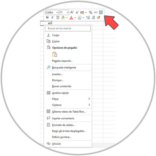
Or we can click on the menu option that says “Format cells”.
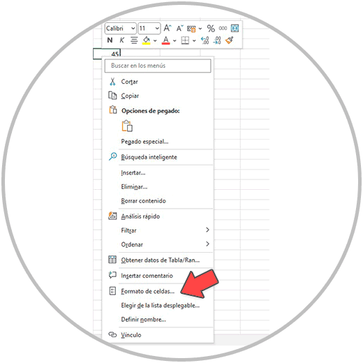
Once we open "Format Cells" a window opens with which we can give the desired format to our cell or range of cells.
- We would have a third option that would be applying a format from another cell. That is, if we have, for example, a cell where we have already applied a currency cell format, we can copy that format and paste it into a cell or range of cells where we want to apply that currency format. In order to copy and paste the format from one cell to another, as we already know, we copy a cell using the Ctrl + C keys on our keyboard, or we would click on the cell where the format to be copied is with the right mouse button. In the options we would select “copy”.
Then, from the “Start” menu, on the ribbon, we click on paste, and then we would select paste format, as in the image below.
Summary:
As we have seen, in order to use Excel, we must first learn the "where" are the most useful options and tools that we are going to need. And then we'll have to learn how we can start entering data into cells, and how we can format cells correctly, depending on the information the cells contain. Thus we can apply currency format, generic numbers, decimals, percentages or dates.
In addition, knowing how to apply formats, in order to learn to use Excel we have to know how to use formulas and make use of functions. We have explained some examples to start seeing how to use formulas in Excel. And we have explained how we can use the functions to save time, to work more productively and safely in Excel.