The use of Microsoft Excel in its new edition 2019 allows us to manage in a much more comprehensive and accurate each data stored in the spreadsheet regardless of its type (numeric, text, date, etc), which can be sure that the results obtained will be exact according to the given conditions..
One of the most common and, in turn, the most important tasks to be carried out in Microsoft Excel 2019 is the comparison of two columns, which is essential to detect differences or duplicates in the registered data, we can use some methods which will depend on the structure of the data. data hosted in the cells of the spreadsheet.
TechnoWikis will explain how we can perform this task which helps us simplify many work tasks by not repeating existing data in one or another column..
1. How to compare two columns in Excel 2019 cell by cell
This method includes the option to execute the search cell by cell automatically through a simple formula. In this case we will use the SI formula, which is integrated in Microsoft Excel and its mission is to make logical comparisons between a value and an expected result.
Step 1
With this SI formula, the instruction we give has two results, first, if the comparison is true and the second if the comparison is false.
The formula to be executed will be the following:
= YES (A2 = B2; "Matches"; "Does not match")
Step 2
In this case, the comparison of cell A2 with B2 is executed and if the result is the same we will get the message Coincides, otherwise we will receive the message Does not match, this result can be dragged to the other cells where it will be carried out. evaluation:
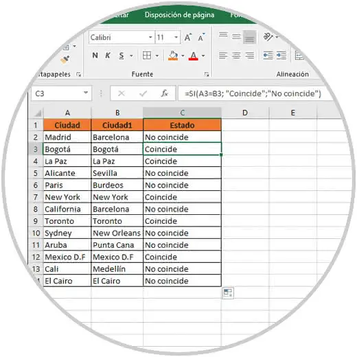
We can see the respective results with their coincidence or not.
Step 3
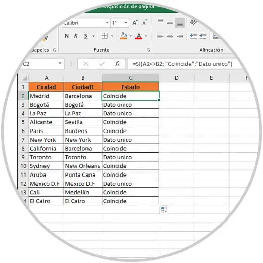
Now, with this function it will be possible to search the different data between the cells of the selected range. In the step we have seen, we have proceeded to search for the same data, if the goal is to find data that is different we will use the following formula:
= YES (A2 <> B2; "Matches"; "Unique data")
In this case the search will be carried out and the data that is different will launch the message Match and the cells whose data are the same will display the message Unique data:
2. How to compare columns case sensitive in Microsoft Excel 2019
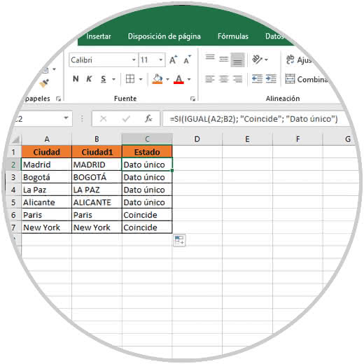
When we record data in Microsoft Excel 2019, it is possible that even though these coincide in your text, some may be uppercase and some may not. It will also be possible to apply a formula that allows us to compare two columns distinguishing between uppercase and lowercase.
In this case, the formula to be used will be the following:
= YES (EQUAL (A2; B2); "Coincides"; "Unique data")
With this formula, all those data that are the same, including lowercase and uppercase, will display the message Match, otherwise we will see the message Unique data:
3. How to compare multiple columns in which their content is equal in all rows Excel 2019
For reasons of content we will not always have only two columns to compare, it is possible that they are more than two and thanks to the formulas of Excel 2019 we can compare them all simultaneously to verify that the content of all of them is identical.
Step 1
For this example we will use 3 cells and the formula to be used will be the following:
= YES (Y (A2 = B2; A2 = C2); "Match"; "Do not match")
As a result, the three cells will be evaluated and we will obtain the message according to the criteria evaluated:

Step 2
If we have several columns to evaluate we must resort to the following formula:
= YES (CONTARSI ($ A2: $ F2; $ A2) = 5; "Match"; "Do not match")
In this case, the number 5 refers to the number of columns to analyze.
4. How to compare values ​​from one column to another in Microsoft Excel 2019
The use of this option allows us to verify that a value registered in column A is in column B, in this case we must use the functions Si and CONTAR.SI as follows:
= YES (COUNTIF ($ B: $ B; A2) = 0; "Does not apply in column B"; "Applies")
Thus, if the value of A is in B we will see the message Apply, otherwise we will see Does not apply in column B:

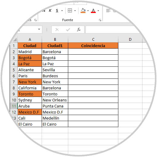
5. How to detect matches in two cells in the same Excel row 2019
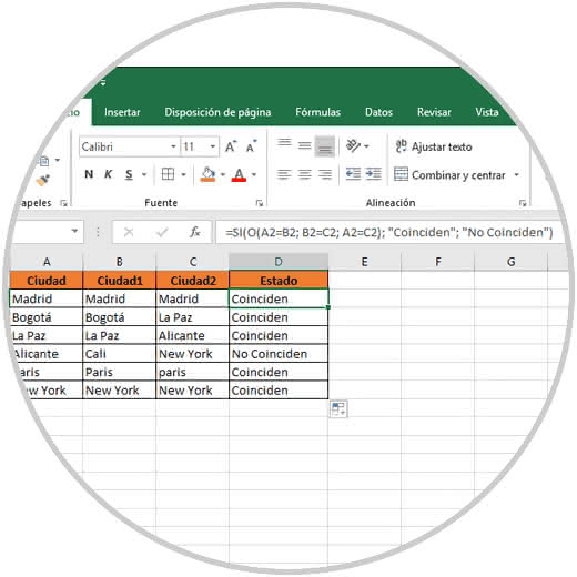
Within the various options of using Excel 2019 formulas, we have the opportunity to detect matches in at least two cells in the same row and not in all the cells. For this task we must resort to the functions Si and O like this:
= YES (O (A2 = B2; B2 = C2; A2 = C2); "Match"; "No Match")
This will evaluate each of the cells of the selected range and based on the data entered there will return the correct message:
6. How to compare data between columns and extract specific data in Microsoft Excel 2019
When using Excel 2019 it is normal that many of the data are in different columns and it is necessary to obtain a specific data lodged in one of those columns. The most useful way to achieve this is by using the VLOOKUP function which can automatically extract the value from the column as we indicated, but in Excel 2019 we can also use the functions INDICE and COINCID in order to obtain the same result.
For this case we will use the following formula:
= INDEX ($ B $ 2: $ B $ 7; MATCH (D2; $ A $ 2: $ A $ 7; 0))
This formula will go to cell E2 using the range of zones B2: B7 and based on the cities registered in the A2: A7 range, if any city in column D does not exist in that range we will see the error # N / A:

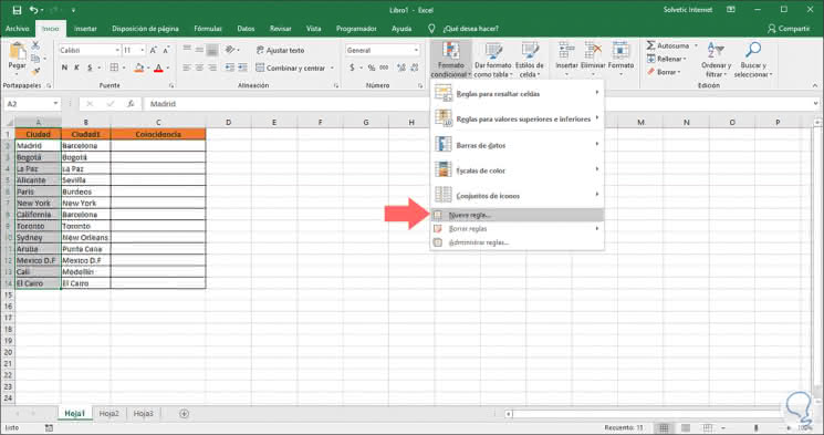
7. How to compare columns and highlight matches found in Excel 2019
It is a practical utility thanks to which the results that coincide will be highlighted which will give us a better visualization of the final results that are detected.
Step 1
For this function we must select the cells to highlight, go to the Start menu and there, in the Styles group, click on the option Conditional Format and in the options we choose New rule:
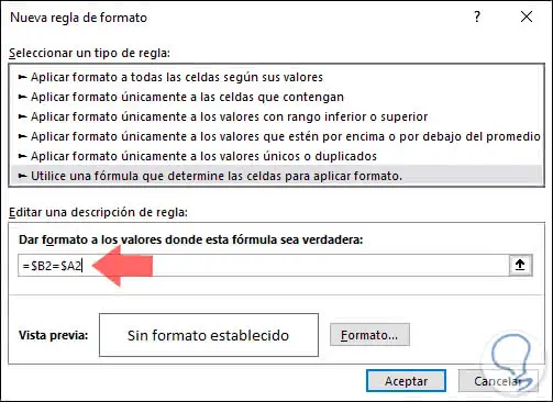
Step 2
The following window will be displayed where we select the option Use a formula that determines the cells to apply format and in the field Format the values ​​where this formula is true enter the following formula:
= $ B2 = $ A2
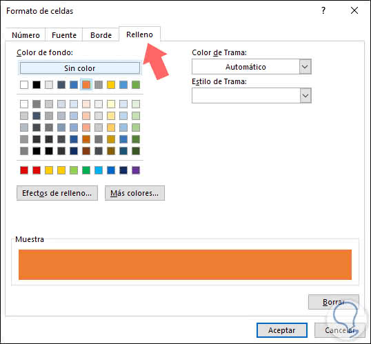
Step 3
There we click on the Format button and on the Fill tab we select the desired color for the highlighting:
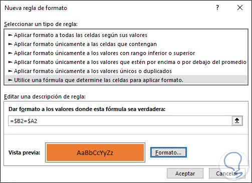
Step 4
Click OK and we will see a preview of it:
Step 5
Click OK to have the format applied to the cells that match the selected range:
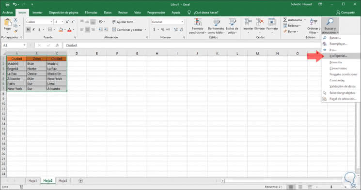
8. How to compare multiple columns and highlight the differences in Excel 2019
Step 1
It is another of the available options thanks to which we highlight the differences this time but not the coincidences. To achieve this we must select the cells to analyze, then go to the "Start menu", go to the "Modify group" and there click on the "Search and select" option and then click on the option Go to "Special"
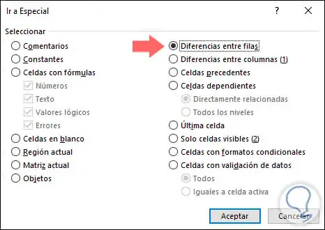
Step 2
The following window will be displayed where it will be necessary to activate the Differences between rows box:
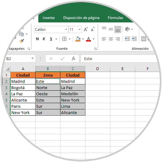
Step 3
Click OK and as a result we can see the cells with different content highlighted in the selected range:
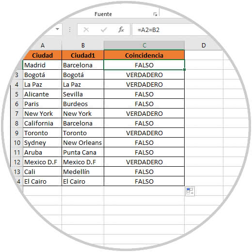
Compare cells using the = sign
One of the most essential ways to determine the match between two columns is using the equal sign (=), for this we simply enter the following:
= A2 = B2
Drag the formula to the other cells and the values ​​that match will have the TRUE legend and otherwise FALSE:
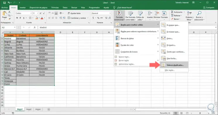
9. How to compare two columns and highlight matches with Excel 2019 format
Step 1
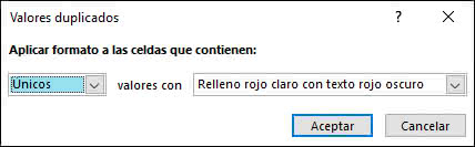
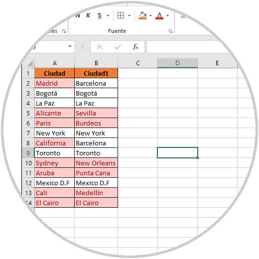
We have already seen how to highlight matches between two columns using a rule, but the conditional format in Excel 2019 integrates an automatic function for that purpose. To make use of it, if we want to use this method, we select the range of cells and in the Start menu we go to the "Styles group" and there we click on the option "Conditional format" where we click on the line "Rules to highlight cells" and in the options displayed select "Duplicate values"
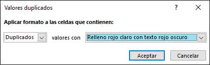
Step 2
In the pop-up window we confirm that the Duplicates option is selected and on the right side we define the color to use for its result:
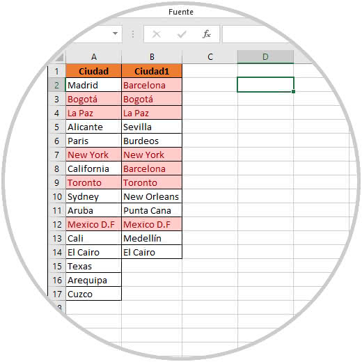
Step 3
Click OK and we will see that the duplicate values ​​will be highlighted in the Excel sheet 2019:
Note
Through this option we can also highlight the unique values, in this case instead of selecting Duplicates we will select Unique:
By clicking on Accept the result will be as follows:
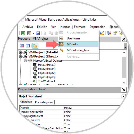
10. How to compare Excel 2019 columns using a Visual Basic macro
Automation is one of the critical points in Excel since it saves us time by avoiding the execution of a repetitive task, but it will also be possible to create a macro to evaluate the matches between two columns.
Step 1
To create this macro, we will use the Alt + F11 keys and in the expanded window we go to the Insert / Modules menu:
Step 2
In the new window we will paste the following code:
Sub Find_Matches () Dim CompareRange As Variant, x As Variant, and As Variant 'Set CompareRange equal to the range to which you will 'compare the selection. Set CompareRange = Range ("C1: C5") 'NOTE: If the compare range is located on another workbook 'or worksheet, use the following syntax. 'Set CompareRange = Workbooks ("Book2"). _ 'Worksheets ("Sheet2"). Range ("C1: C5") ' 'Loop through each cell in the selection and compare it to 'each cell in CompareRange. For Each x In Selection For Each and In CompareRange If x = and Then x.Offset (0, 1) = x Next and Next x End Sub 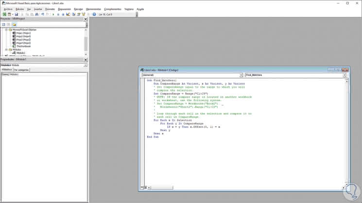
Step 3
Again we use the Alt + F11 keys to return to Microsoft Excel and now we go to the Progaramador menu and there we select the values ​​of column A and then click on the Macros option:
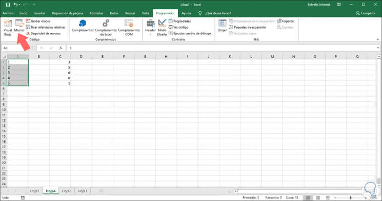
The following will be displayed:
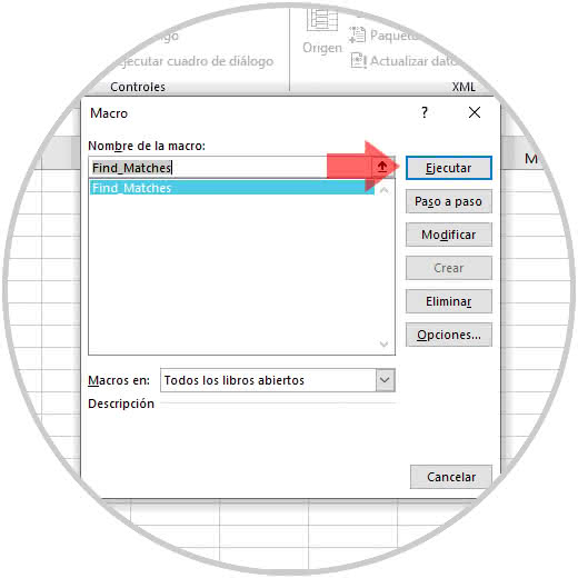
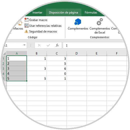
Step 4
There we click on Execute and as a result the duplicate numbers will be displayed in column B, the matching numbers will be placed next to the first column:
As we can see, the alternatives to manage the duplicate values ​​in Microsoft Excel 2019 are varied and each one has its own editing conditions, it depends on us to select the most suitable one..