Although the Excel name for many can become synonymous with fear and complexity, it is not if we have the right knowledge. However, thanks to this spreadsheet tool , we have the possibility to perform different actions in a simple way, thanks to the large number of formulas that we can apply to manage data..
Microsoft Excel is really a practical utility for the complete and integral management of the data to work and one of the actions that we most frequently execute in Excel 2019 is to compare data from the cells . Something so simple but that can lead to many problems since the comparison of data is ideal for determining the integrity of a data in Excel.
TechnoWikis will explain some methods to compare both data and columns in Excel 2019 and thus manage in a much more centralized way..
1. Compare columns using the cell-by-cell method in Excel 2019
Step 1
As the name implies, this method is responsible for executing the search through each cell by cell in a fully automatic process. In this case we have the following information:
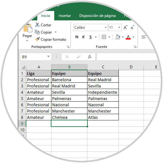
There we will add a new column where we will register if the data matches or not, in this case it will be in column D and in cell D2 we enter the following formula:
= YES (B2 = C2; "Matches"; "Does not match")
Step 2
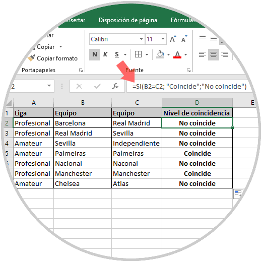
What we do with it is that the value of cell B2 is compared and if it is the same as the value of cell B3 the message “Match†will be launched, otherwise we will see the message “Does not matchâ€:
Step 3
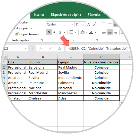
Now, it is possible to search for different data between cells. Different to look for the same data, if we want to search only the different data we will use the following formula:
= YES (B2 <> C2; "Matches"; "Does not match")
2. How to compare columns between upper and lower case in Excel 2019
Many times when we manage data in Excel 2019, column data can be either lowercase or uppercase. Therefore, if we want to visualize the same data, it does not matter if it is in content or in writing, we will use the following formula:
= YES (EQUAL (B2; C2); "Matches"; "It is a unique value")
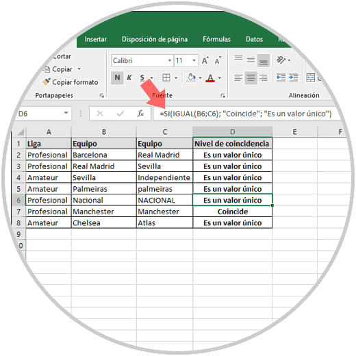
There we can observe that, although some data are the same, their difference lies in the uppercase or lowercase which makes it different.
3. How to compare multiple columns in Excel 2019 where their content is the same in all rows
Another of the options offered by Excel 2019 is the possibility to see if the data registered in their cells are identical or not. For this task it will be necessary to combine the Si and Y functions simultaneously, in this example we will execute the following:
= YES (Y (B2 = B3; B2 = D2); "Match"; "Don't match")
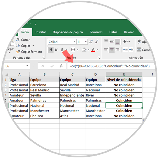
There we can observe that a comparison is made between all the columns and only the "Match" message is given where all the values ​​are identical..
If we have a large number of columns to analyze, we can execute the following:
= YES (CONTARSI ($ B2: $ H2; $ B2) = 8; "Match"; "Don't match")
There the number 8 refers to the number of columns to analyze.
4. How to find matches in two cells in the same row in Excel 2019
Excel 2019 gives us the opportunity to find matches in at least two cells of the same row but not in general in all the cells of the workbook, for this we must combine the Si and O functions like this:
= YES (O (B2 = C2; CB2 = D2; B2 = D2); "Match"; "Not Match")
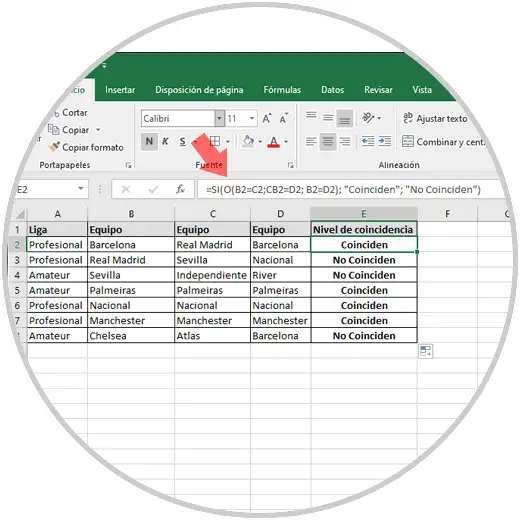
We can see that where the same term is twice the message "Match" will be displayed, if it does not match in any row we will see "Do not match".
5. How to compare values ​​from one column to another in Excel 2019
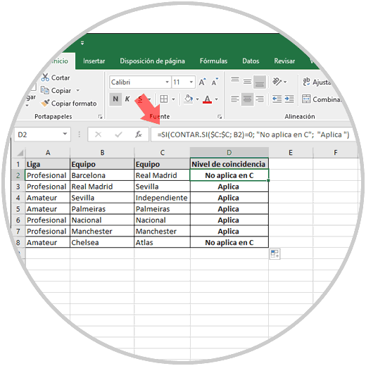
Now, we may want to compare whether the value of column A or B is in column B or C, in this case we must use the functions Yes and COUNT.SI as follows:
= YES (COUNT IF ($ C: $ C; B2) = 0; "Does not apply in C"; "Applies")
When executing this formula, if the data in cell B is present in column C we will see the message “Appliesâ€, otherwise we will see the message “Does not apply in Câ€:
6. How to compare data between columns and extract specific data Excel 2019
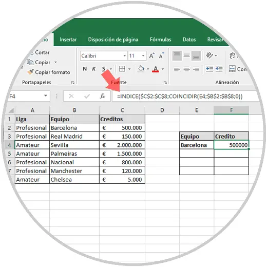
Some data in Excel 2019 can be distributed in different columns so that the use of the VLOOKUP function is ideal to access this data, but in Excel 2019 we can use the INDEX and MATCH functions to obtain this information exactly.
In this example, we want to obtain the credit granted based on the name we enter in cell E4, and there we will use the B2: B8 data range for the query, the formula to be used will be the following:
= INDEX ($ C $ 2: $ C $ 8; MATCH (E4; $ B $ 2: $ B $ 8; 0))
This formula is recorded in cell F4 and the name is entered in cell E4 and there we will obtain the result:
7. How to compare columns and highlight matches in Excel 2019
This is a much more ideal method to visualize the coincidences since it will be possible for the cells where the respective values ​​are applied to be highlighted thanks to the cell format.
Step 1
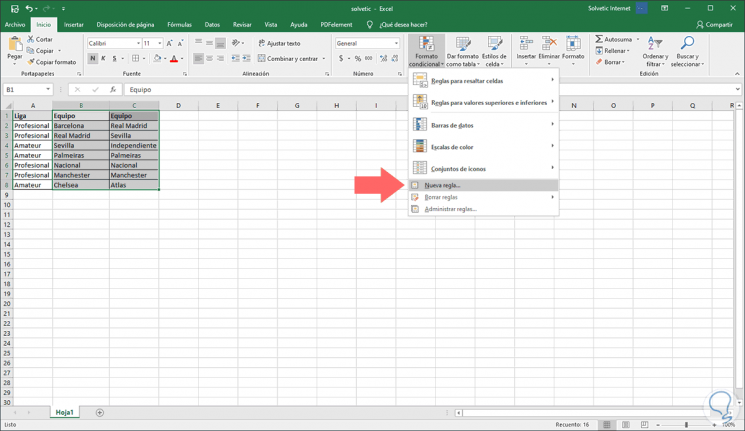
If we want this method we must select the range of cells to highlight and go to the "Conditional formatting" option located in the "Styles" group and in the options displayed we choose "New rule":
Step 2
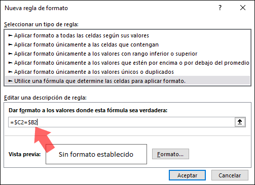
In the displayed window we select the line “Use a formula that determines the cells to apply format†and in the field “Format the values ​​where this formula is true†enter the following formula:
= $ C2 = $ B2
Step 3
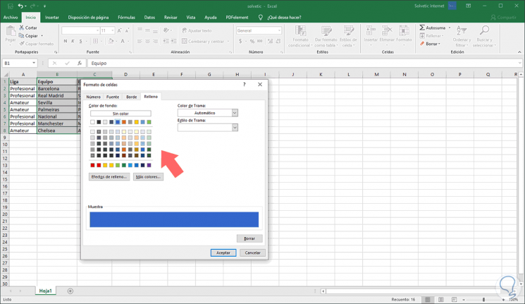
To set the highlight, we click on Format and then choose the desired color from the “Fill†tab:
Step 4
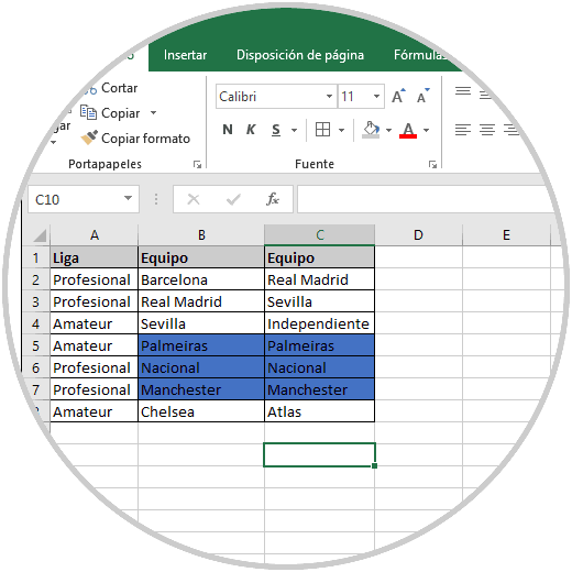
Click OK to view the results:
8. How to compare multiple columns and highlight the different ones in Excel 2019
This will be possible with a special Excel 2019 function associated with the special paste.
Step 1
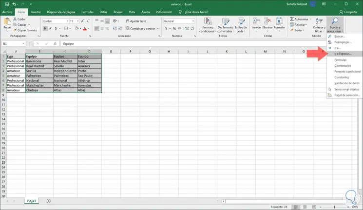
To make use of it we will go to the Start menu, Edit group, click on Search and select and there we will click on the Go to Special option but first select the cells to analyze:
Step 2
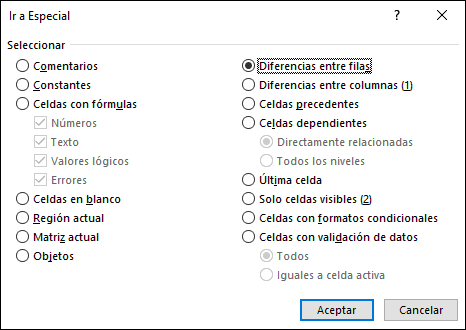
In the wizard that will be displayed, we must activate the “Differences between rows†box:
Step 3
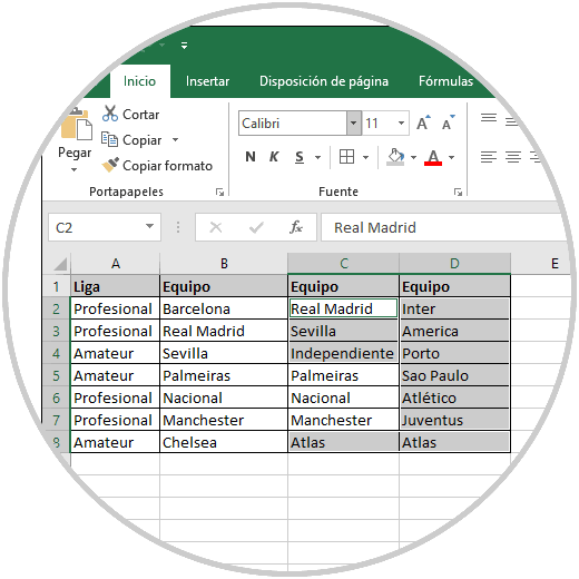
By clicking on Accept we can visualize the different data in the selected range:
9. How to compare dates in Excel 2019
If you are a frequent user of Excel 2019 you will have noticed that the dates are one of the most used data in Excel and with which more errors can be presented by the format of the same, but if you want to compare dates in Excel to determine which is greater than another , TechnoWikis will give you the answer in a simple way.
Step 1
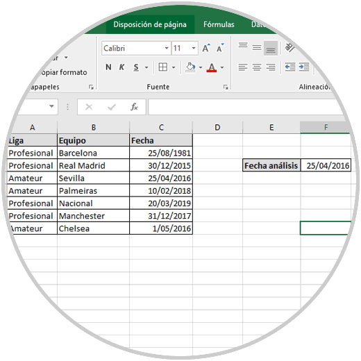
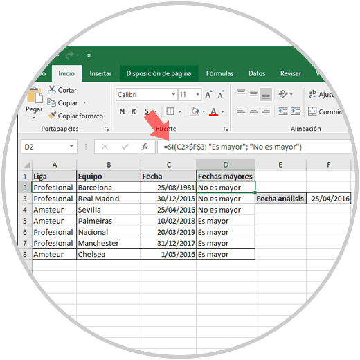
For this example we have a range of dates in column C and we will take a base date (cell F3) in order to compare which dates are greater than this:
In order to execute the comparison we will enter the following formula:
= YES (C2> $ F $ 3; "It is greater"; "It is not greater")
Step 2
There, we have established the base cell (F3) as an absolute value so that when comparing column C with that cell we will see that if the date is less or equal the message “It is not greater†will be displayed but if the date is greater we will see "Is older":
We see how the handling of Excel 2019, although it seems something extreme, with TechnoWikis it is something simple and fun with which obtaining the necessary information will not become an ordeal.