Microsoft Excel 2016 and 2019 are one of the most used applications thanks to its versatility, security and performance for the management of large amounts of data in a simple, but at the same time precise, hence the importance of being exactly each of them. your options in terms of functions, formulas and tools for the administration of these. Undoubtedly, Microsoft Excel provides us with hundreds of options, whether unique or combined, in which the work of the data will be carried out precisely and one of these options is the use of logical functions..
The basic purpose of the logical functions is to make a decision based on the given criteria, thus, a logical function first of all analyzes the fulfillment of a given condition and taking as a point of reference the result, it will decide whether or not to execute the objective action. TechnoWikis will do a complete analysis of five of the most used logical functions in Microsoft Excel and for this case we will use Excel 2019 but the same process will apply in Excel 2016.
1. How to use SI function in Microsoft Excel 2019 and Excel 2016
Thanks to the SI function it will be possible to carry out a logical comparison between a value and the required result by executing an analysis of a condition and based on this the SI function will return the expected result if the condition is true or false.
Based on this instruction, the SI function will have only two results, which are:
- The first result is that if the comparison of the results meets the conditions, it will be True.
- In case any of the conditions does not meet the requirements your result will be False.
We can use the IF function combined with logical functions such as Y, O and NO and in this way we can execute evaluations with the given conditions..
Some of the syntax to use with the IF function, combined or unique, are:
YES (Y ()): YES (Y (logical_value1, [logical_value2], ...), value_if_true, [value_if_false]))
YES (O ()): YES (O (logical_value1, [logical_value2], ...), value_if_true, [value_if_false]))
YES (NO ()): YES (NO (logical_value1), value_if_true, [value_if_false]))
The arguments that we should use with the SI function in Microsoft Excel are:
logical_test
It is a mandatory value which means the value that we are going to evaluate
value_if_true
It is another mandatory value which refers to the value that will be returned in case the result of the evaluation is TRUE.
value_if_false
It is an optional value which allows us to generate a result in case the value returned from the evaluation is FALSE.
To understand its structure a little better we are going to make some practical examples.
Step 1
In this first example, we will use the following condition in which it is explained that, if cell A2 is greater than B2, True will be returned, otherwise the value returned will be False:
= YES (A2> B2; TRUE; FALSE)
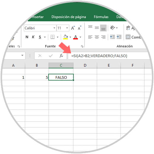
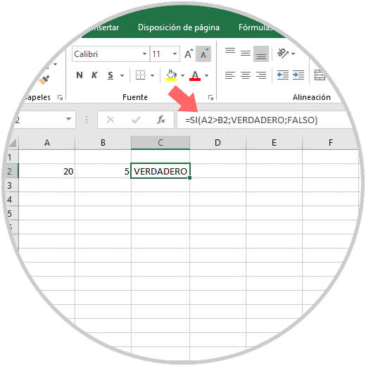
Step 2
Now, if the condition meets the parameters, the result will be true:
Step 3
The SI function can be applied to various conditions such as:
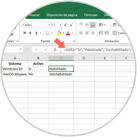
Text
It is possible that based on the answer in a cell its result is evaluated, for example, in column B we have entered if a system is active or not, the IF function will evaluate that if the system is active it will launch the Enabled message, otherwise the message will be disabled, the function to be used will be:
= YES (B2 = "Yes"; "Enabled"; "Disabled")
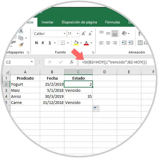
Dates
This can cover several variables, an example is to determine if an item has expired and if it is not knowing how many days it is due to expire.
For this case we will combine the SI function together with the TODAY function:
= YES (B2 <HOY (); "Expired"; B2-HOY ())
Thus, the products that have already expired will have the legend expired and those that we will not see the number of days remaining until their expiration:
Step 4
By using the IF function, and most Excel logical functions, it is possible to use logical operators, these are:
- <=: less than or equal to
- > =: greater than or equal to
2. How to use the nested SI function in Excel 2016 and Excel 2019
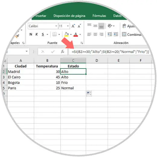
Microsoft Excel allows us to nest an IF function, that is, use another SI function in the same original function, to understand this we will perform an analysis where we will analyze the time status based on criteria such as high, normal or low.
For this case we will use the following nested formula:
= YES (B2> = 30; "High"; YES (B2> = 20; "Normal"; "Cold"))
Thus, temperatures greater than or equal to 30 will be high, from 20 to 29 will be normal and otherwise they will be cold:
3. How to use IF function with conditional format Excel 2016 and Excel 2019
The conditional formats are another of the options that integrate Excel 2016 and 2019 through which it will be possible to create and edit rules that when they are met, a certain format option will be applied when the criteria used is met.
Step 1
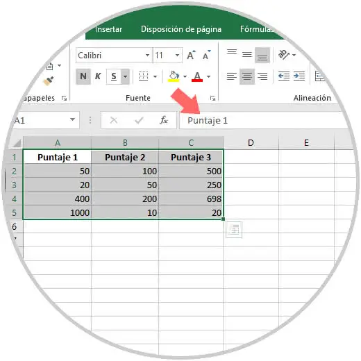
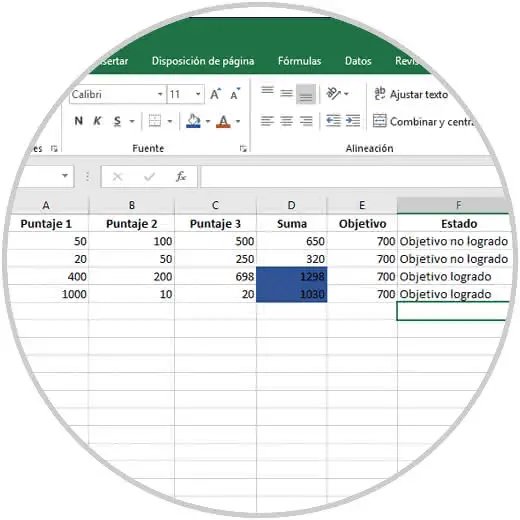
For this example we are going to highlight the cells whose value in column D is greater than the value in column E and to use the conditional format we will first select the data to be evaluated:
Step 2
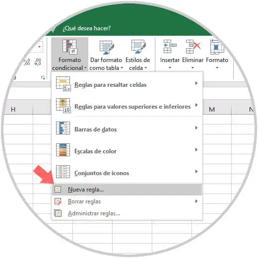
Then, we go to the Start menu and in the Styles group we click on the option Conditional Format and we will select New rule:
Step 3
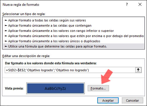
In the expanded window we will go to the section Use a formula that determines the cells to apply format and in the field Format the values ​​where this formula is true enter the following formula:
= YES (D2> E2; "Goal achieved"; "Objective not achieved")
Step 4
To apply the format we click on the Format button and in the next window we go to the Fill tab and there we will select the desired color:
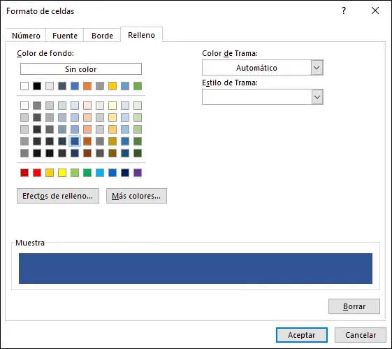
Step 5
It will also be possible to edit the font, borders, etc. We press OK and automatically the condition will be applied in the cells that fulfill this analysis:
4 How to use the O function in Microsoft Excel 2016 and Excel 2019
The function O in Excel has the task of determining if some of the conditions entered in a cell are TRUE.
The OR function will generate the TRUE message in case any of the arguments entered meets the criteria and is evaluated as TRUE, if it is not, its result will be FALSE only if all its arguments are analyzed as FALSE.
Step 1
Its basic usage syntax is the following:
O (logical_value1, [logical_value2], ...)
The arguments to use with the OR function in Microsoft Excel 2016 or 2019 are:
Logical_value1
It is a mandatory value since this is the condition that will be used to validate that the status of the data entered is TRUE or FALSE.
Logical_value2
It is an optional value and refers to the additional conditions that can be added to test the data as TRUE or FALSE, it supports up to 255 conditions.
Some aspects to consider with the O function are:
- Arguments must be evaluated as logical values, such as TRUE or FALSE, matrices or references whose contents are logical values ​​are also compatible.
- If in the range we have entered no logical values ​​are detected, the O function will return the error value # VALUE !.
- If any of the cells in the range to be evaluated have text or empty cells, these values ​​will not be analyzed.
- It is possible to use an O matrix formula to check whether a value appears in an array or not.
Some examples of how to use the O function in Excel are as follows..
Step 2
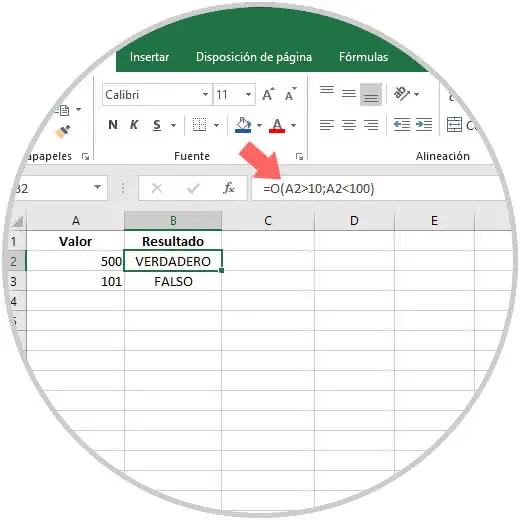
A simple example is the following, in cell A2 we have entered a value which will be analyzed with the following formula:
= O (A2> 10; A2 <100)
If the number is greater than 10 but less than 100, its result will be True, otherwise it will be False:
Step 3
Also with the OR function we can analyze several cells, for example, if cell B2 is greater than or equal to 3000 and cell C2 is greater than or equal to 6, the result will be True, otherwise False:
= O (B2> = 3000; C2> = 6)
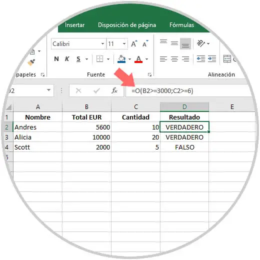
With the OR function, both criteria must be met so that the result is False, with only one of the criteria being met, the result will be True.
Step 4
Using the IF function with O, it is possible to combine both logical functions to obtain a result in Microsoft Excel, for this we have the following information:
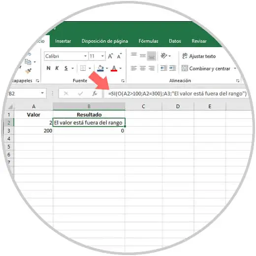
= YES (O (A2> 100; A2 = 300); A3; "The value is out of range")
There, the value of cell A3 will be displayed if its value is greater than 100 O if it is equal to 300, otherwise we will see the message "The value is out of range":
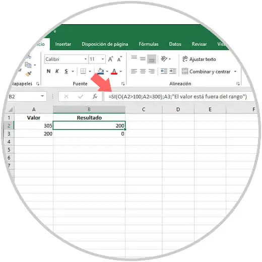
Step 5
Now, if we add a value greater than 100 or equal to 300 we will see in cell B2 the value of cell A3:
5. How to use the NO function in Microsoft Excel 2016 and Excel 2019
It is another of the most used functions in Excel 2016 and 2019 and its use is basically to determine that one value is not equal to another.
Its usage syntax is:
= NO (logic)
It is normal that the function is NOT combined with others to increase the analysis capabilities of other Excel logical functions and thus achieve better results.
The only argument of this function is NOT the following:
Logical_value
It is a mandatory value and indicates a value or an expression which must be evaluated as TRUE or FALSE.
We have mentioned that the function DOES NOT invert the value of the result since, if the logical value is FALSE, the function will NOT return TRUE and if the logical value is TRUE, the function does NOT return FALSE.
Step 1
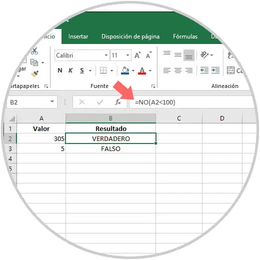
A simple example of this function is the following:
= NO (A2 <100)
There, if the value of cell A2 is less than 100, it will NOT return True so the number is greater, otherwise its value will be False:
Step 2
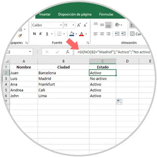
It will be possible to combine the SI function with the NO function, for this in this example we will use the following formula:
= YES (NO (B2 = "Madrid"); "Active"; "Not active")
As a result, the cells where the Madrid value is the result will be Not Active and in the others its result will be Active:
Step 3
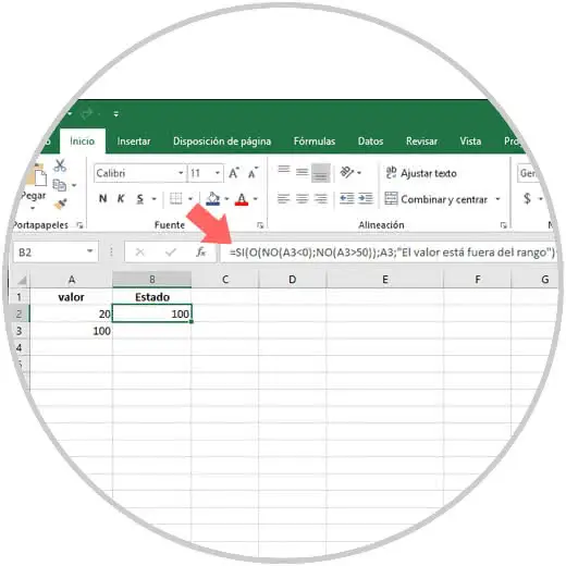
Another example to use will be with the following formula:
= YES (O (NO (A3 <0); NO (A3> 50)); A3; "The value is out of range")
Step 4
There we will have two values ​​that are 20 (A2) and 100 (A3), we know that 100 is not less than 0 (FALSE) and 100 is greater than 20 (TRUE), but the OR function will invert this logic of the arguments TRUE / FALSE. The OR function only requires that one of the arguments be TRUE for its analysis:
6. How to use the Y function in Microsoft Excel 2016 and Excel 2019
Another of the most used functions of Excel 2016 and 2019 is the AND function which determines if all the conditions in an analysis are TRUE to yield the expected results.
In a practical way, the AND function will return the TRUE result if all the arguments have the parameter TRUE and FALSE in case one or more arguments are analyzed as FALSE.
Its usage syntax is:
= Y (logical_value1, [logical_value2]
The arguments to use with this Y function are the following:
Logical_value1
It is a necessary value since it is the condition that will be used to evaluate the data as TRUE or FALSE.
Logical_value2
It is optional since they indicate the additional conditions to be tested and that can be TRUE or FALSE, the Y function supports up to a maximum of 255 conditions.
To consider:
- If the specified range does not contain logical values, the Y function will return the error # VALUE!
- If there are empty cells or text, they will not be analyzed by the Y function
Step 1
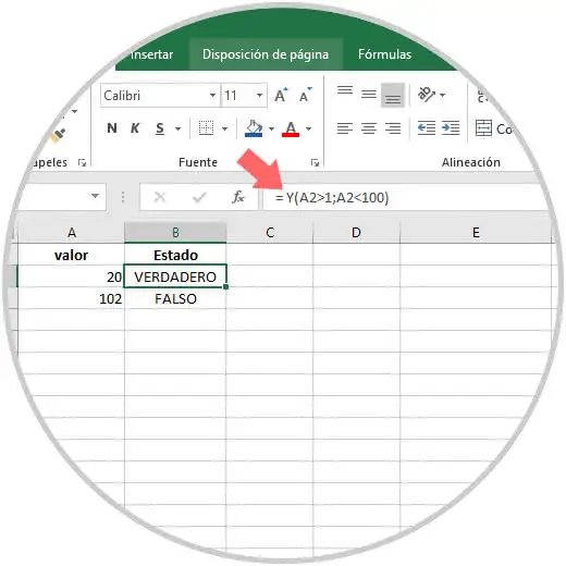
A practical example is to execute the following.
= Y (A2> 1; A2 <100)
Step 2
There, the result will be TRUE if A2 is greater than 1 and is less than 100, otherwise the result will be FALSE:
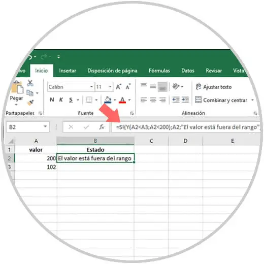
Now we will use the following formula:
= YES (Y (A2 <A3; A2 <200); A2; "The value is out of range")
Step 3
There, we will see the value of cell A2 if it is less than A3 and it is less than 200, otherwise we will see the message "The value is out of range":
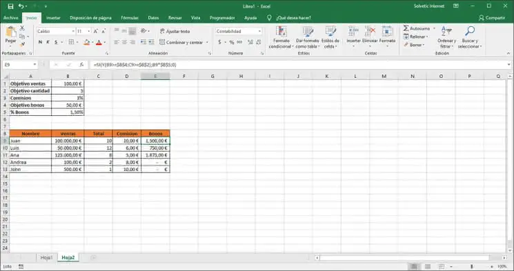
Step 4
Now, a useful example of the function Y, linked with another logical function such as If is to execute the following:
= YES (Y (B9> = $ B $ 4; C9> = $ B $ 2); B9 * $ B $ 5; 0)
This is a commission environment where the SI function will analyze the Sales value and if it is greater than or equal (> =) to the Sales target, and the Total value is Higher or Equal (> =) than the Target amount, it will multiply the value of Sales for the% of Bonds, otherwise the value will be 0:
7. How to use the XOR function in Microsoft Excel 2016 or 2019
The function XOR (English) or XO (Spanish) of Excel, is a function which will return a logical exclusive OR of all the arguments analyzed.
Step 1
Its usage syntax is:
= XO (logical_value_1, [logical_value_2])
The only argument to use is:
Logical_value1, logical value2
The logical_value1 is mandatory, and the following logical values ​​are optional, the XOR function supports from 1 to 254 conditions to check if a condition is TRUE or FALSE and can be logical values, matrices or references.
Some aspects to keep in mind when we use XO are:
- The result of XO will be TRUE when the number of TRUE entries is odd and FALSE when the number of TRUE entries is even.
- If the evaluated range does not contain logical values, the XO function will generate the error value # VALUE!
- In case of finding text or empty cells they will not be analyzed
Step 2
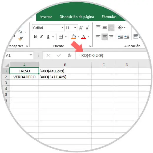
We can use the following basic examples to know how XO acts:
= XO (4> 0.2 <9)
With this line, we see that one of the two conditions is True, the TRUE message will be returned.
= XO (3> 11.4> 5)
Step 3
In this case all the conditions are false, therefore, the result will be FALSE
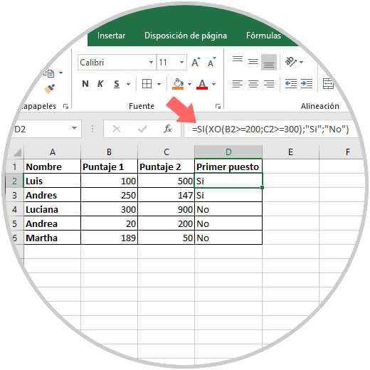
Now, it will be possible to use the XO function next to the SI function, for example, we will enter the following line:
= YES (XO (B2> = 200; C2> = 300); "Yes"; "No")
Step 4
There we will analyze two columns, B and C, and there the XO function will act only if one of the proposed conditions is met.
We check how the logical functions in Microsoft Excel 2016 or 2019 will be of great help to execute multiple calculations with precision and with the best features that Excel gives us.