Microsoft Excel is one of the most used suites in the world for managing large amounts of data of various types such as text, number, dates, etc. This means that it would be a more complex task if we did not have the functions and integrated Excel formulas for it..
Currently we are near Excel 2 019 which will have new and improved functions but for anyone it is a secret that when using an Excel spreadsheet we have hundreds of tasks that we can execute either to organize the information or for the user Accessing the spreadsheet has multiple alternatives to use the data. In this case we can take the drop-down lists to allow both us and the users who use the spreadsheet to select the most appropriate option or answer according to the need.
Drop-down lists are cells that include the possibility of selecting different options within the same cell. This is really useful when we want users to fill out forms or surveys using a list of options that we have created. This drop-down list draws on a range of cells with values ​​that we have defined..
TechnoWikis will explain how we can create a drop-down list in Microsoft Excel 2019.
1. Create a drop-down list in Excel 2019
To create and configure a drop-down list in Excel 2019 we can use the data validation function in order to create drop-down menus in Excel cells. As a requirement it will be necessary to have a list of data and an input cell of data.
Step 1
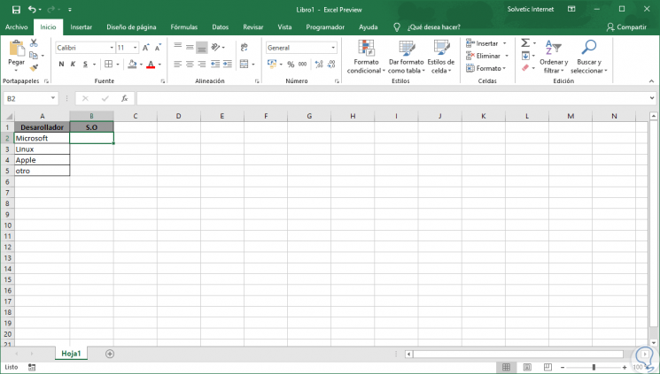
To create the drop-down list in the Excel 2019 cell, we must list the entries that must appear in the main menu, for this we can use any range of data, and in addition to this we must select the cell where the drop-down list will be created, in In this case we will use the range A2: A5 and the cell where the list will be inserted will be cell B2:
Step 2
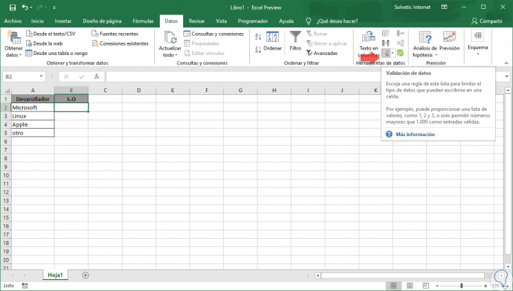
Now we will go to the “Data†menu and in the “Data tools†group we will find the “Data validation†option:
Step 3
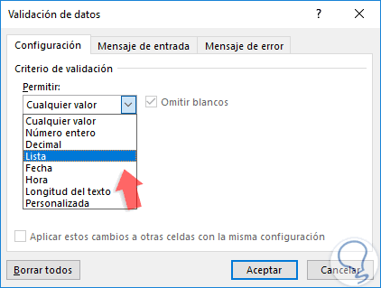
Clicking on this option will display the following pop-up window where we will select the "List" option in the "Allow" field:
Step 4
Once this option is selected, the “Origin†field will be activated where we must select the range of cells where the options to select from the drop-down list in Microsoft Excel 2019 will be available:
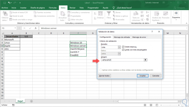
Step 5
It is important to activate the following boxes:
Skip targets
In order to discard empty cells.
Cell with drop-down list
So that these answers are with this format.
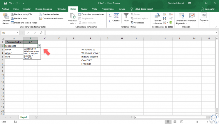
Step 6
Click on the "Accept" button and we can see that in the cell from where the data validation was generated, a drop-down list has been inserted, which if we click we can see the options of the selected origin range. There we can click on any of the available answers to complete the process.
2. Display a text input message in the drop-down list in Excel 2019
One way to customize access to the data in the drop-down list is to add a message to guide users about the purpose of the drop-down list.
Step 1
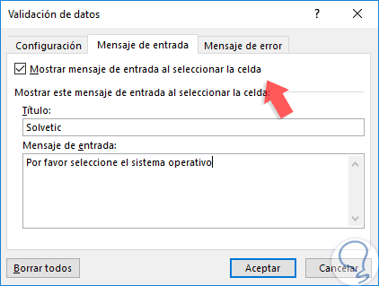
To insert this message, we go back to the "Data validation" option and this time we will go to the "Incoming message" tab and there we configure the following:
- Check the box “Show this input message when selecting the cellâ€.
- Enter the title of the message in the "Title" field.
- We enter the desired message in the "Incoming message" field.
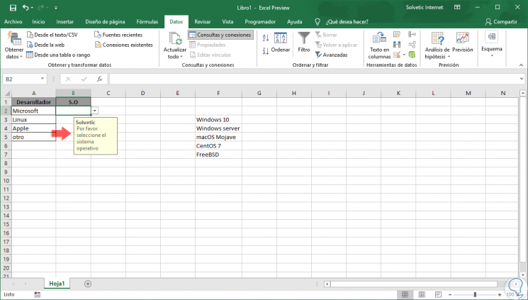
Step 2
Once this is configured, click on the "Accept" button. So, when we click on the cell we will see the following:
3. Display alerts or errors in the cell for incorrect data in Excel 2019
This option allows an error or a warning to be displayed when trying to enter a value that is not within the established origin range.
Step 1
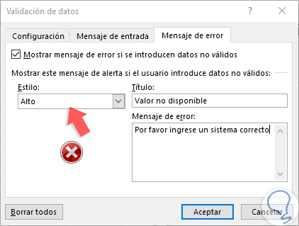
To create this message, we go back to the "Data validation" option and this time in the "Error message" tab we define the following. Alternatively we can define a style as High or Warning.
- Check the box "Show this alert message if the user enters invalid data".
- Enter the title of the message in the "Title" field.
- We enter the desired message in the "Error message" field.
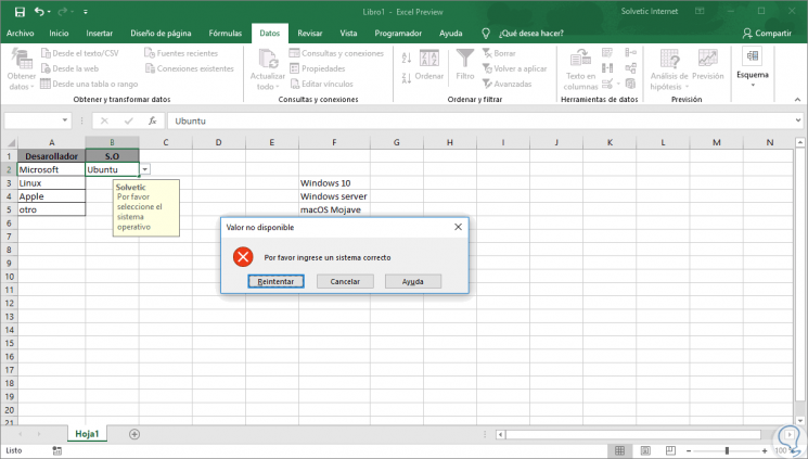
Step 2
Click on Accept and in this way, if the user enters a data that is not in the list, the following will be displayed:
Thus, the drop-down lists in Excel 2019 give us the opportunity to improve the use of information and validate that users enter the established parameters..