Excel is one of the most versatile applications for working with data of various types (date, text, numbers) and in large quantities thanks to its various functions and formulas that have been integrated to deliver precise results, but in addition to this there are some options to manage the information and one of these is to make use of drop-down lists which allow the user to select an answer from a menu of options without altering the result, it is ideal for surveys or exams, TechnoWikis will explain how to create a drop-down list in Excel in a simple way ..
By creating a drop-down list in Excel we can include information related to options or lists to choose different elements. This can help us to show and hide information and thus, in the same space, propose different options. That is why we are going to see how to make this checklist and thus be able to have a list of options in Excel.
To stay up to date, remember to subscribe to our YouTube channel!
SUBSCRIBE ON YOUTUBE
How to create dropdown list Excel
Step 1
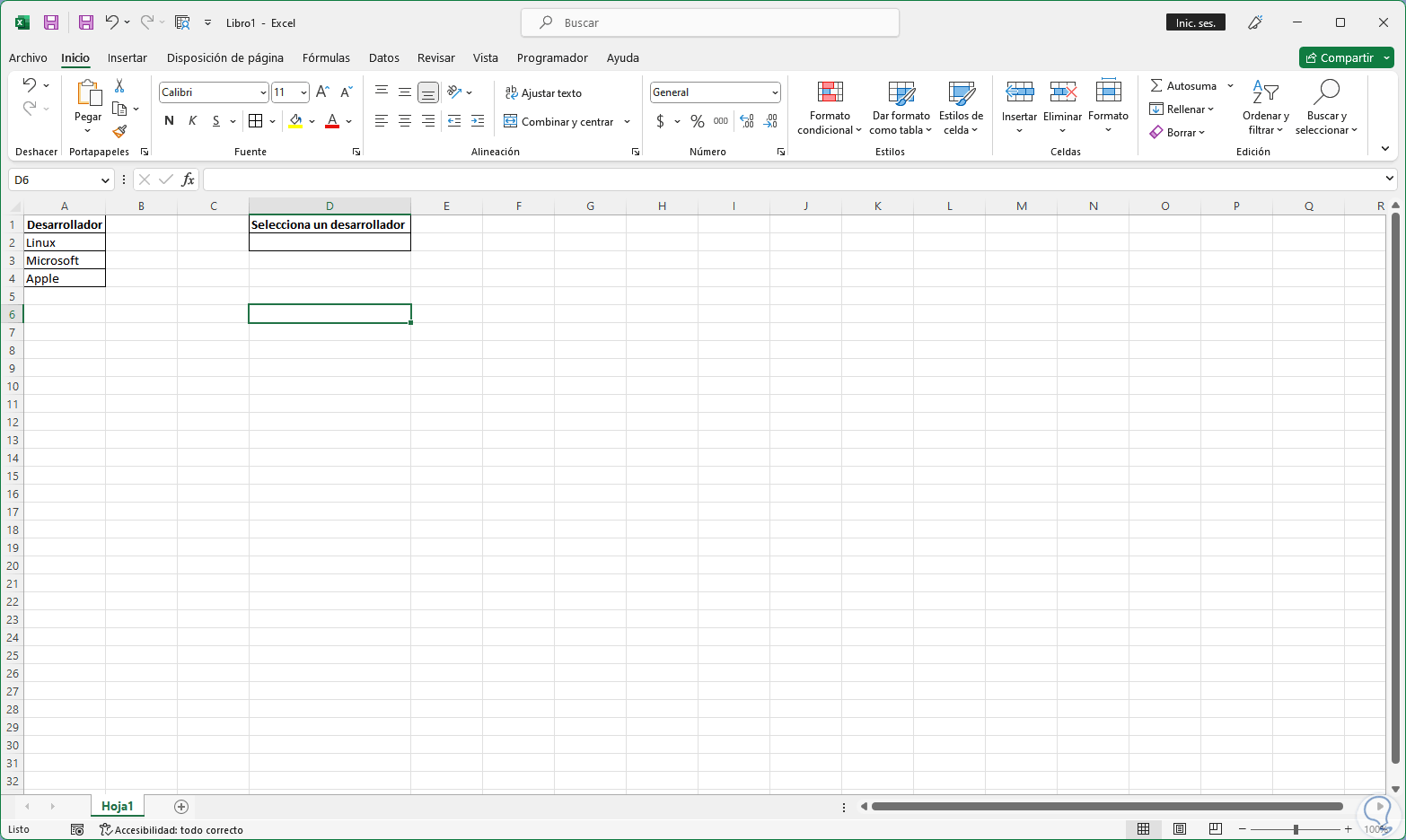
Open Excel and check the data to use:
Step 2
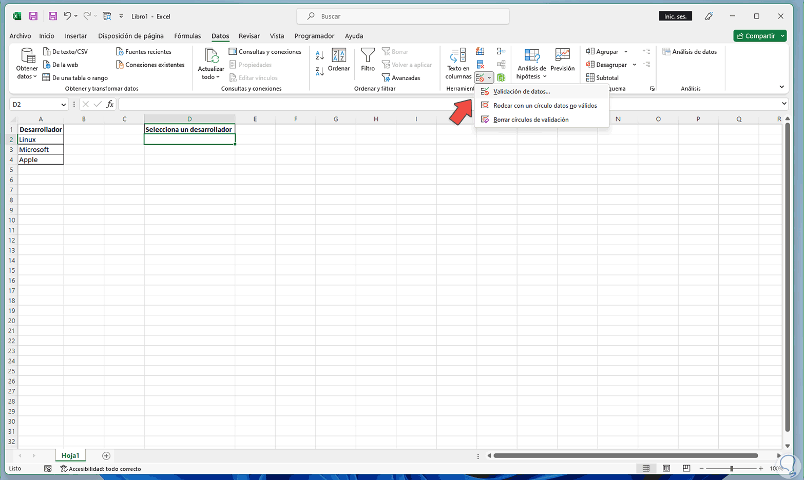
Select the cell where the drop-down list will be, then go to the "Data" menu and there click on "Data validation":
Step 3
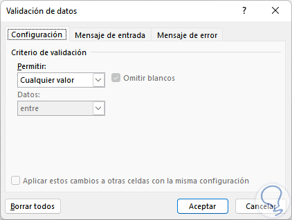
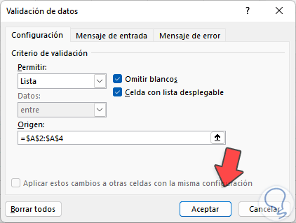
The following will open:
Step 4
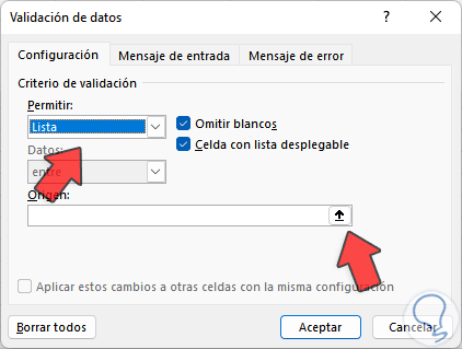
Under "Allow" select "List":
step 5
Select the data to display in "Origin":

step 6
We can see the selected range. Apply the changes.
step 7
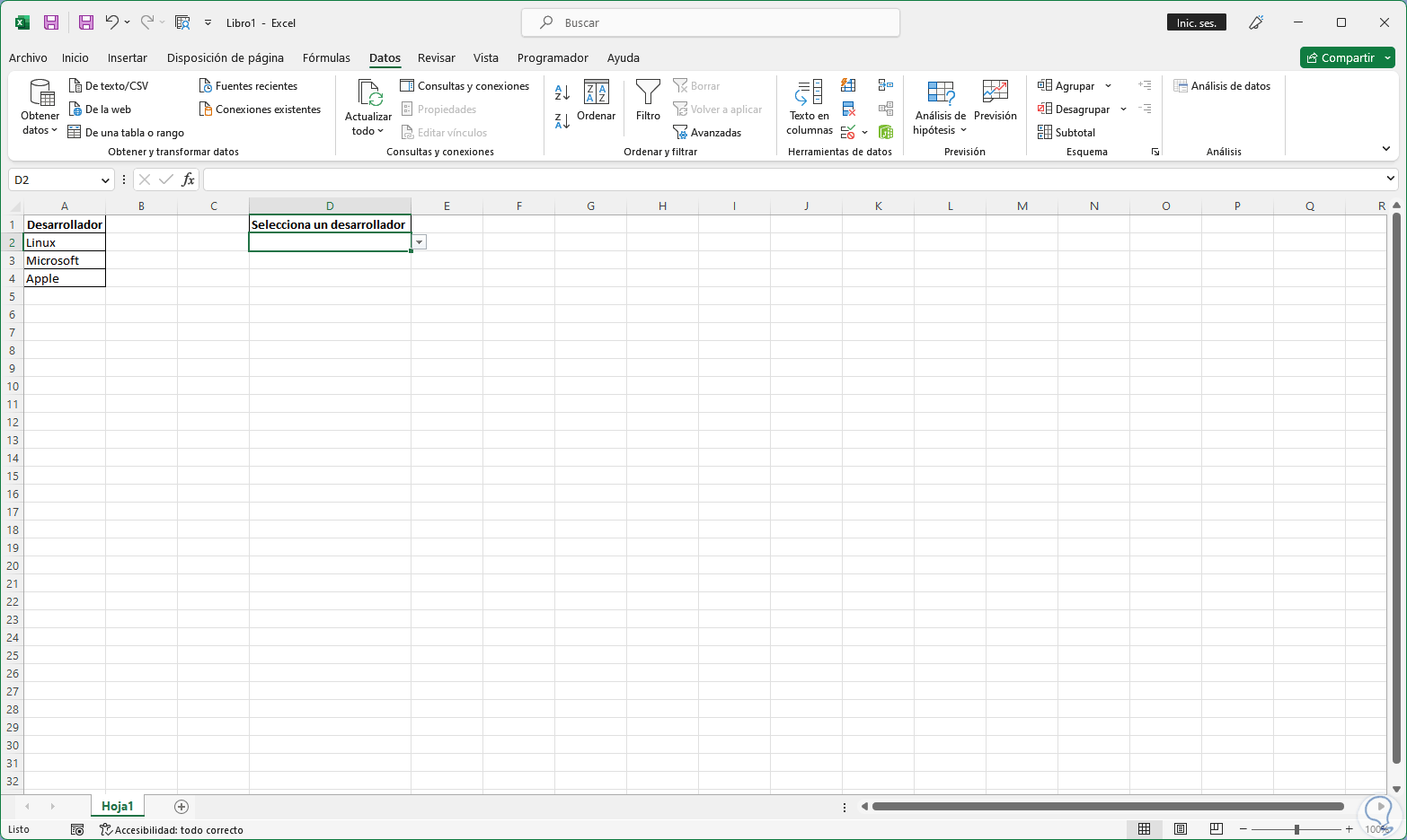
We will see the arrow in the cell that has been selected:
step 8
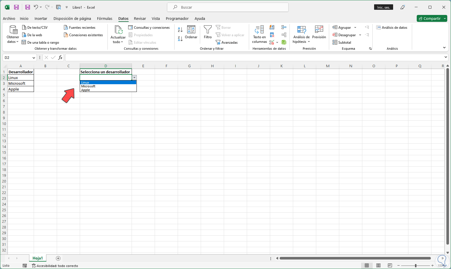
We click on the drop-down arrow and it is possible to choose one of the available values:
step 9
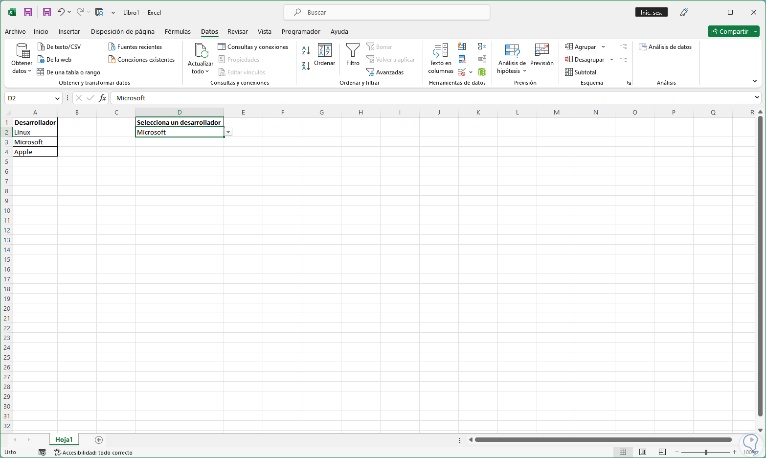
We click on the desired value:
step 10
In case of manually entering a wrong value we will receive a notification alerting:

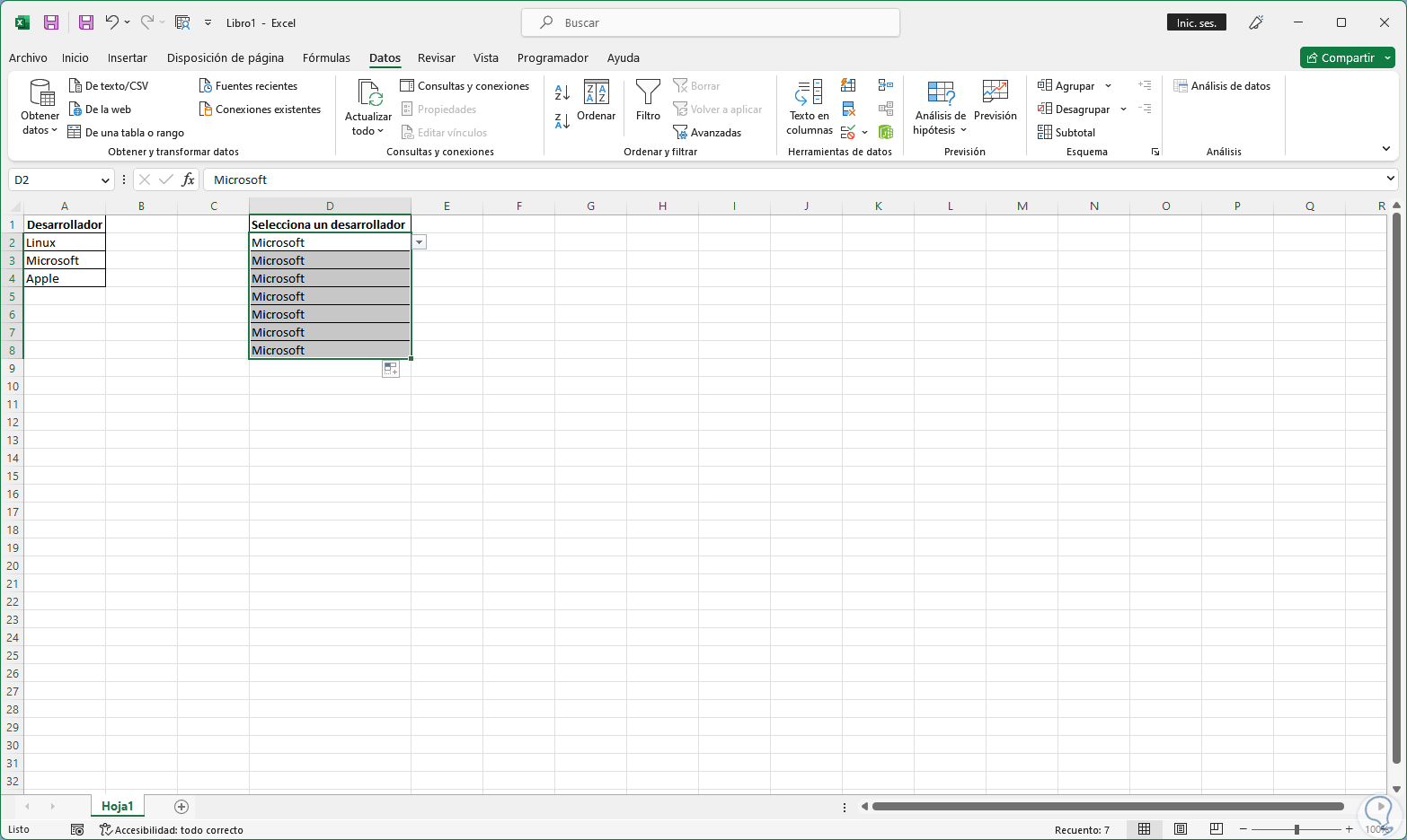
step 11
Drag this cell if you want the list to be available in more places:
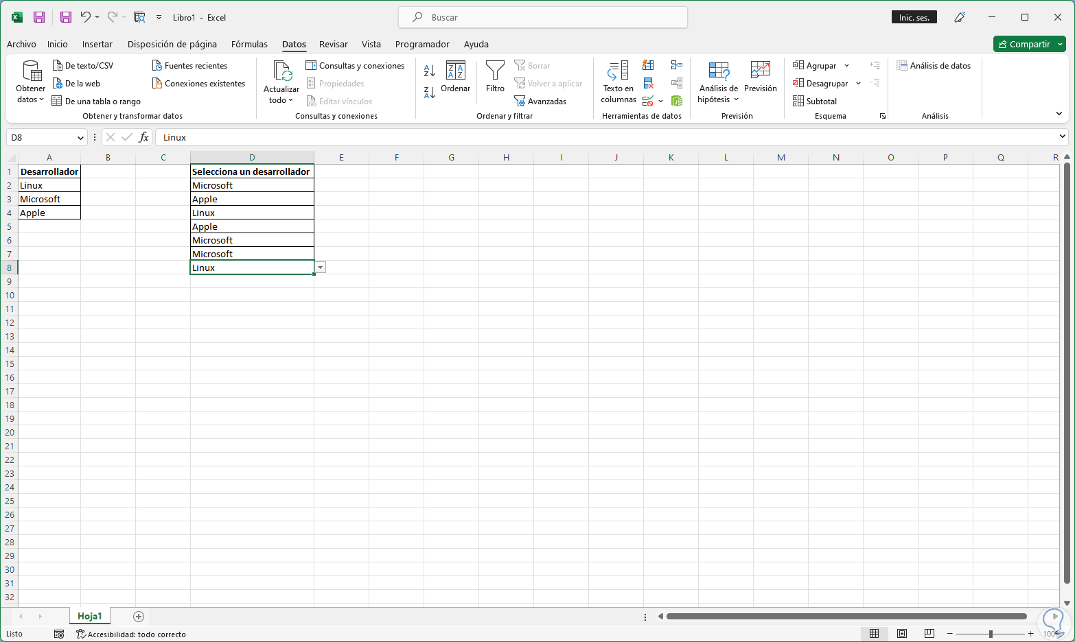
step 12
There we will be able to select the desired values from the drop-down list:
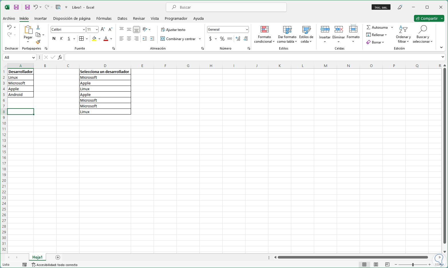
step 13
It is possible to add more data to the list:
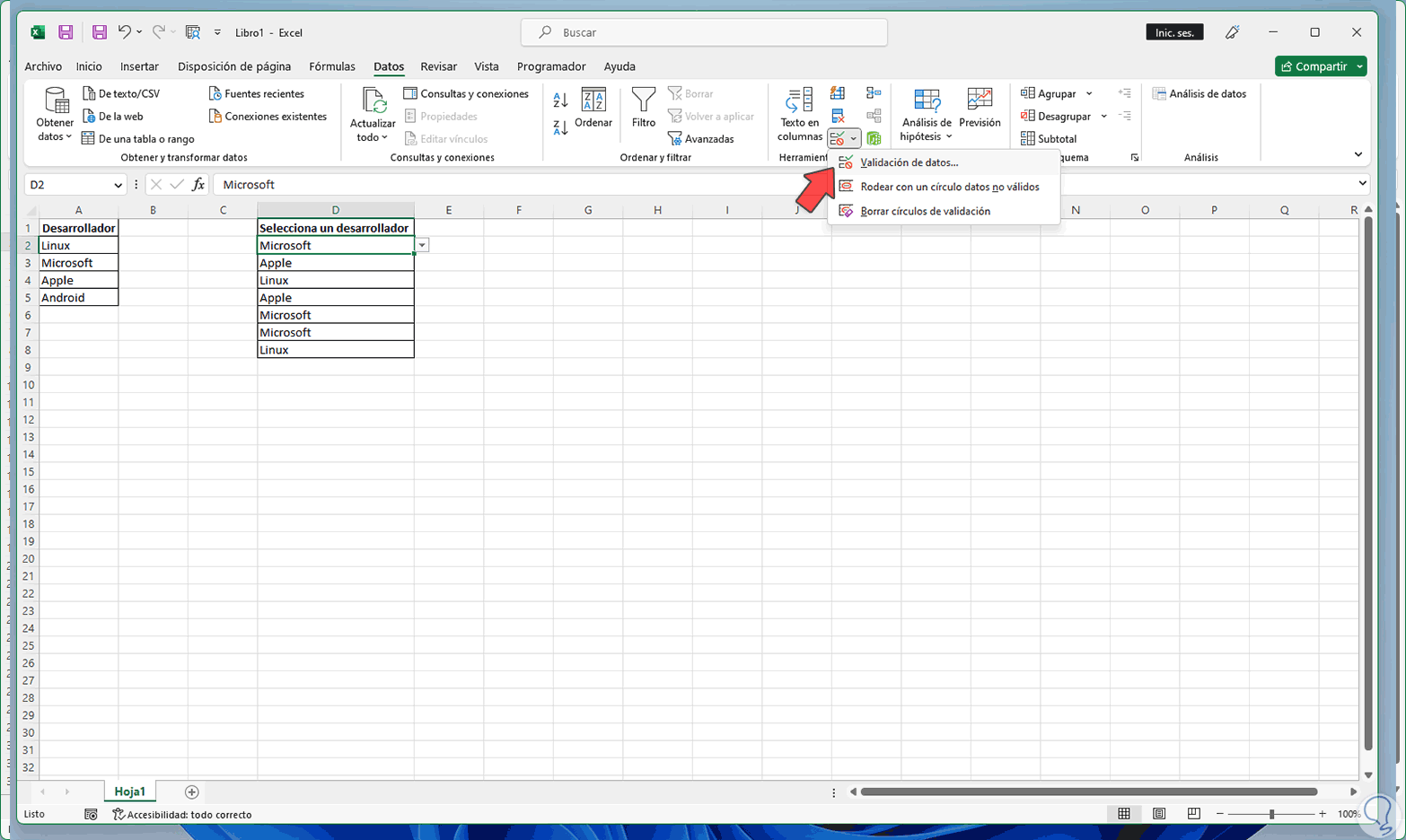
step 14
Once the data is entered, open "Data validation":
step 15
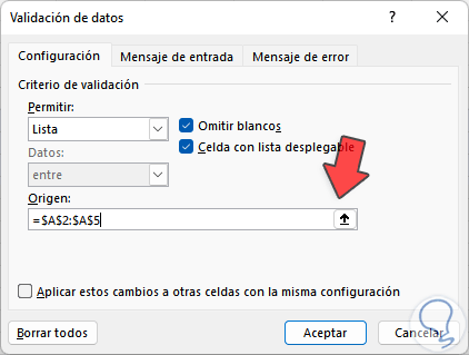
Set the data source: Applies the changes.
step 16
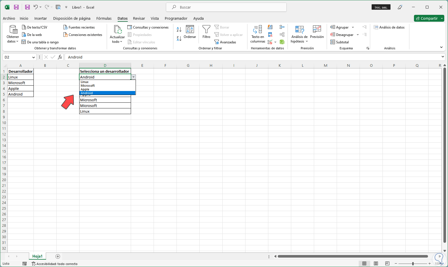
Now that new data will be available in the drop-down list:
Note
Drag the cell to the others to have the update.
step 17
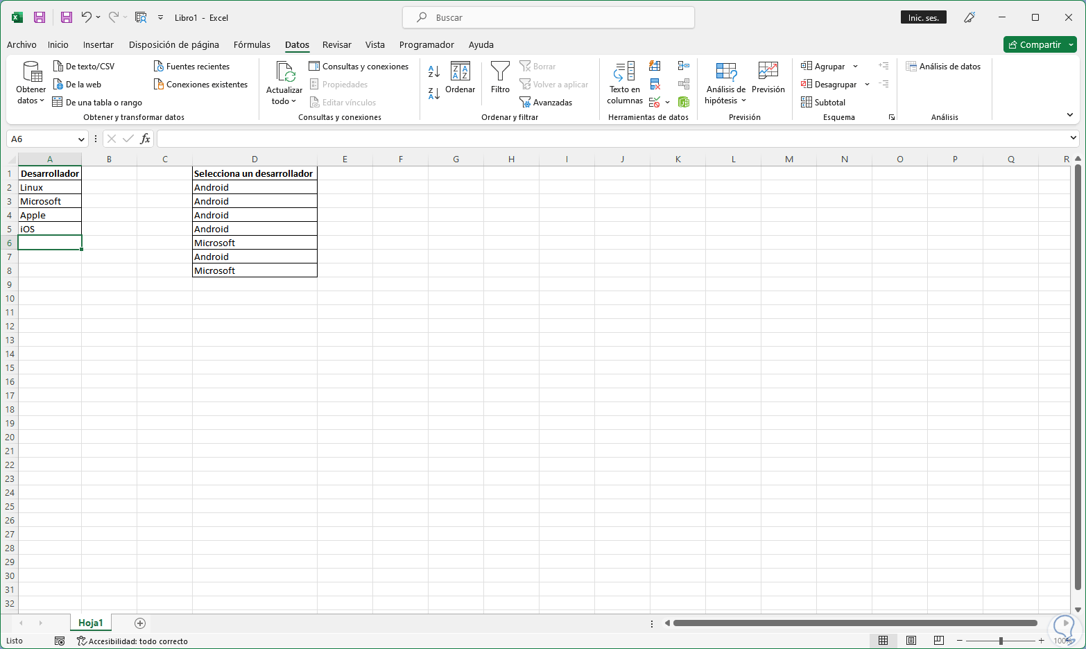
You can change a name on the source directly:
step 18
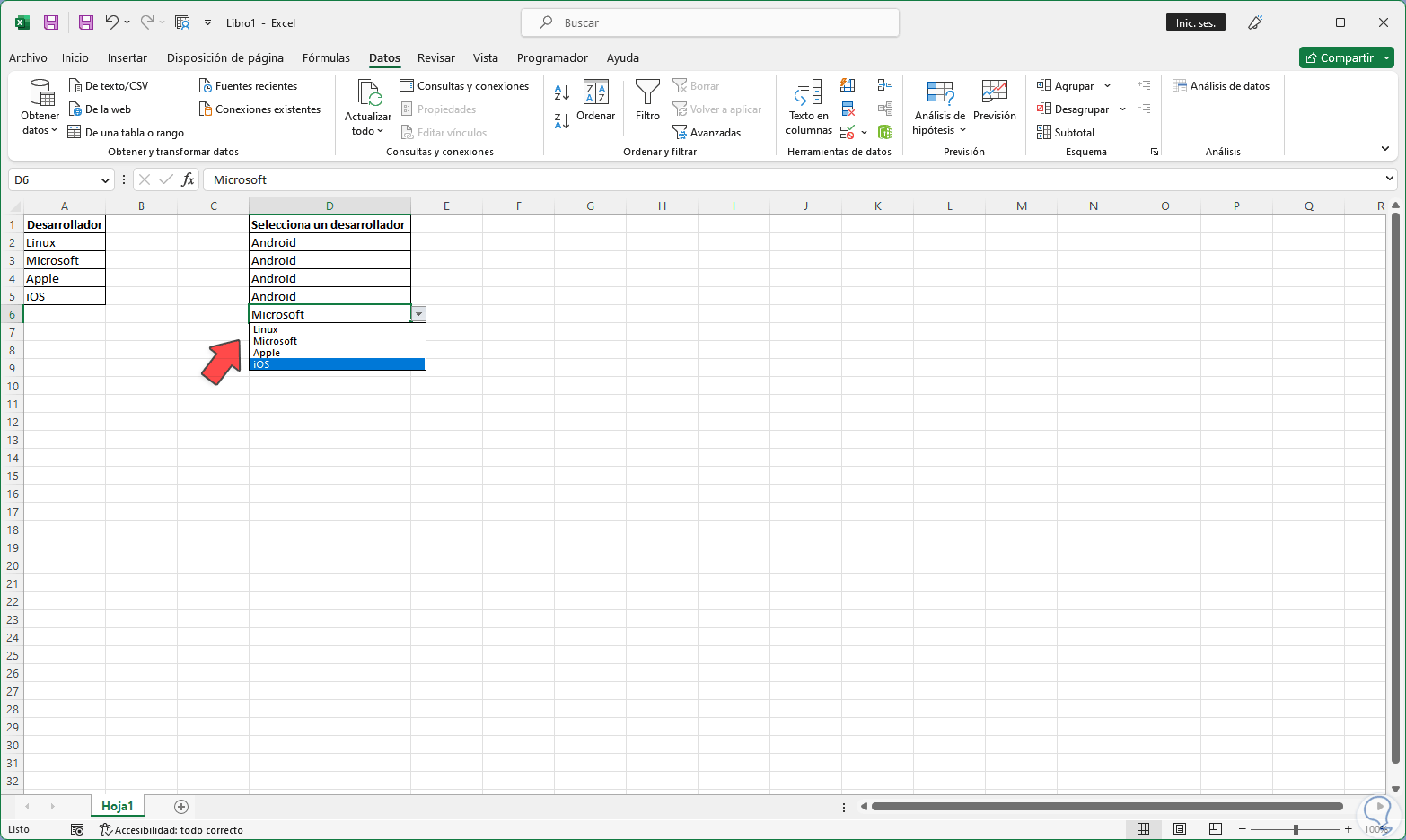
This will automatically update in the dropdown list:
step 19
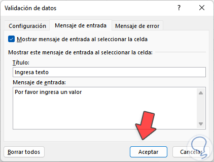
Open "Data validation", it is possible to enter an input message for the user to orient:
step 20
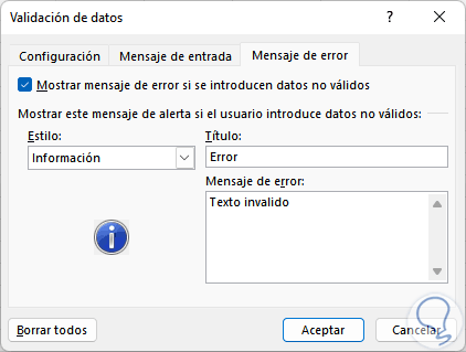
It is also possible to enter an error message to customize the user experience:
step 21
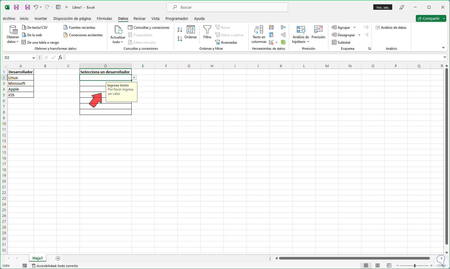
In the cell of the drop-down list we will see the message:
step 22
In case of entering wrong text we will see the defined message:

Step 23
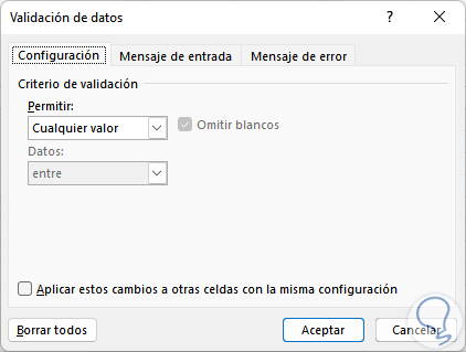
To clear the dropdown list open "Data Validation":
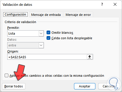
Click on "Delete all":
step 24
We see how the parameters change, apply the changes.
step 25
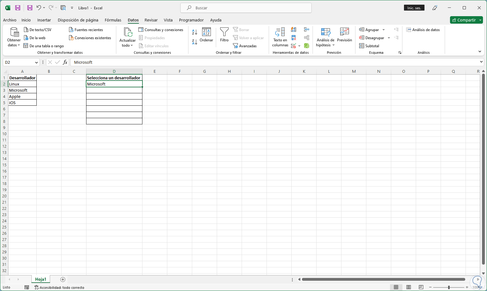
We validate that the list will not be available.
This is the easy way to create a dropdown list in Excel and be able to better manage the supplied data..